Exponential Moving Average on Streaming Data

tl;dr: The exponential moving average is more responsive to recent data than the cumulative moving average, and unlike the cumulative moving average, it is not vulnerable to floating point precision problems as the amount of data increases.

I’ve written about the cumulative moving average in a previous article. In this article, I’ll explore a variation on this idea known as the exponential moving average.

In a comment, edA-qa pointed out that the cumulative moving average still poses precision problems as values are added.

As we will see, the exponential moving average does not have this problem. It also has the potentially useful property that it is more responsive to more recent values.

The formula for the exponential moving average is a special case of the weighted moving average.

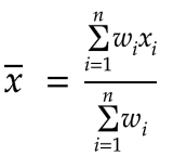
The weighted average is a variation on the simple average. The simple average is the sum of each value (the total), divided by the number of values (the count). With the weighted average, we multiply each value by a number that we call its weight and add these products up for the total. Then we divide by the sum of all the weights. The higher the weight for a given value, the more it will contribute to the weighted average. If we assign 1 as the weight for each value, then the weighted average just reduces to the simple average. The formula for the weighted average is:

I won’t show the full derivation of the recurrence relation for the weighted moving average. If you’re interested, the details are in Tony Finch’s excellent paper Incremental calculation of weighted mean and variance. The derivation is very similar to that of the cumulative average that we’ve already gone through.

We’ll start with the recurrence relation for the weighted moving average:

Compared to the formula for the cumulative mean, instead of multiplying by 1/n, we’re multiplying by the ratio of the most recent weight to the total weight.

w_n is the weight of the nth value, x_n. W_n is the sum of all of the weights:

What happens if we set the ratio w_n/W_n to a constant that we’ll denote by the Greek letter alpha (α)?

We define alpha to be between 0 and 1 (non-inclusive):

Having defined alpha, we can now substitute it into our weighted mean formula:

This is the recurrence relation for the exponential moving average. As far as the basic logic goes, that’s all there is to it! We’ll continue a bit further so that we can understand the properties that result from choosing to define α = w_n/W_n.

We can implement this logic in code as follows:

class ExponentialMovingAverage {
	constructor(alpha, initialMean) {
		this.alpha = alpha
		this.mean = !initialMean ? 0 : initialMean
	}

	update(newValue) {
		const meanIncrement = this.alpha * (newValue - this.mean)

		const newMean = this.mean + meanIncrement

		this.mean = newMean
	}
}

A few questions come up:

• What does alpha do?
• What value should we set alpha to?

To help explore these questions, we’ll apply a few changes to our recurrence relation.

First let’s multiply out alpha in the second and third terms on the right:

Rearranging the order, we get:

We know that:

We can substitute this into our equation to obtain:

This form of the equation is quite useful! We can see that the most recent value has a weight of alpha, and all of the previous values are adjusted to the complementary weight, 1-alpha. Let’s say that alpha is 0.7. The most recent value will have a weight of 0.7. In other words, it will contribute to 70% of the average. All of the previous values will contribute a total of 1 - 0.7 = 0.3, or 30% to the average.

We can define this complementary constant, 1 - alpha, using the Greek letter beta (β):

Replacing 1-alpha in our equation with beta, we get:

Let’s modify our earlier code to use this version of the formula:

class ExponentialMovingAverage {
	constructor(alpha, mean) {
		this.alpha = alpha
		this.mean = !mean ? 0 : mean
	}

	get beta() {
		return 1 - this.alpha
	}

	update(newValue) {
		const redistributedMean = this.beta * this.mean

		const meanIncrement = this.alpha * newValue

		const newMean = redistributedMean + meanIncrement

		this.mean = newMean
	}
}

Also let’s subclass ExponentialMovingAverage to keep track of the weights that are being used for each new value:

class ExponentialMovingAverageWithWeights
	extends ExponentialMovingAverage{
	constructor(alpha, mean) {
		super(alpha, mean)

		this.weights = [1]
	}

	update(newValue) {
		super.update(newValue)

		const updatedWeights = this.weights.map(w=>w * this.beta)

		this.weights = updatedWeights
		
		this.weights.push(this.alpha)
	}
}

Tracking the weights is for demonstration purposes. It’s probably not desirable in production!

How are the weights distributed? Here’s a graph of the weights after 3 values have arrived, using an alpha of 0.1:

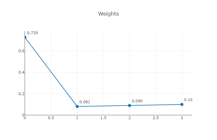
How are these weights calculated?

• We initialize the weights to [1]: This weight will be assigned to whatever the mean is initialized to before any data comes through. If the mean is initialized to 0, then the first weight will not have any effect on the moving average.
• When the first value comes in, we assign its weight to 0.1 (alpha). The previous weights, currently just [1], are multiplied by 0.9 (beta). The result is that we now have weights of [0.9, 0.1].
• When the second value comes along, we assign its weight in turn to 0.1. The previous weights are multiplied by beta. The weights become [0.9 * 0.9, 0.9 * 0.1, 0.1] = [0.81, 0.09, 0.1].
• When the third value arrives, we repeat the process again: We have [0.9 * 0.81, 0.9 * 0.09, 0.9 * 0.1, 0.1] = [0.729, 0.081, 0.09, 0.1].

As we can see, the sum of the weights always adds up to 1.

Let’s take a look at the weights for the first 60 values with an alpha of 0.1:

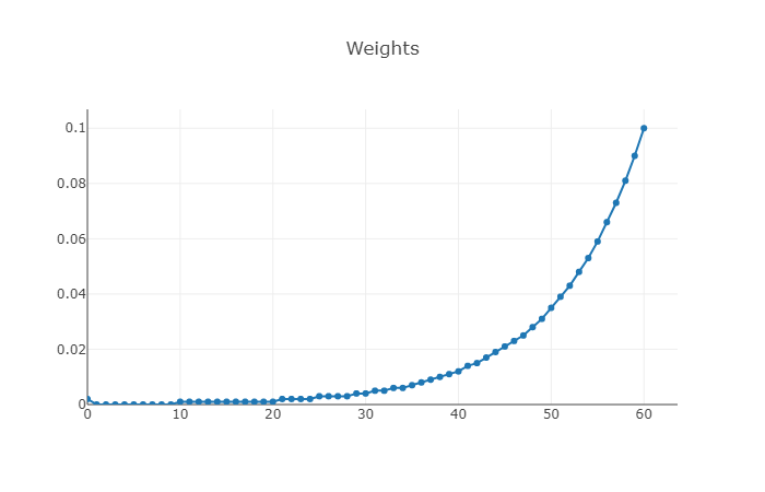
Once the number of values is high enough, we can see that an exponential curve emerges. Alpha is always assigned to the most recent value, and the weights drop off exponentially from there, hence the name “exponential moving average.”

There will always be a small bump on the left side of the curve because we chose an alpha less than 0.5. However, it’s clear from the graph above that this effect becomes insignificant fairly quickly as new values are added.

Let’s see how the weights are affected by several different values of alpha (0.1, 0.5, 0.8):

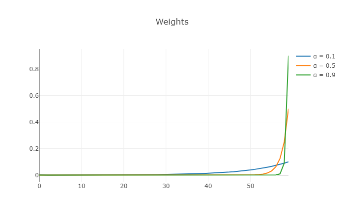
As we can see, the higher the value of alpha, the more weight is placed on the most recent value, and the faster the weights drop off for the rest of the data.

Now let’s have a look at some sample data and compare the exponential moving average (alpha is set to 0.1) with the cumulative moving average:

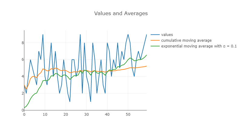
One problem we can see right away is that the exponential mean starts at 0 and needs time to converge toward the cumulative mean. We can fix that by setting the initial value of the exponential mean to the first data value. Alternatively, sometimes the exponential mean is seeded with the average of a larger sample of initial values.

Let’s try it again, this time initializing the exponential mean to the first value:

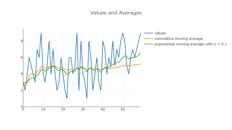
Now we don’t have to wait for the exponential mean to catch up, great!

Let’s try this again, only instead of using an alpha of 0.1, let’s use 0.8:

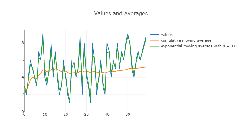
Because we’re weighing the most recent data so heavily in this case, the exponential average tracks the actual data almost exactly rather than following fairly closely to the cumulative mean.

It may be worth noting in passing that while the exponential moving average does not suffer from precision problems as the number of values increases, there could still be an issue with floating points: If the density of the data is very high, we may want to use a value of alpha that’s extremely small, and that could be problematic. The good news is that it’s either a problem or it’s not. It won’t get worse over time.

So, how do we choose a value for alpha? There appear be two ways:

• Find an analytical approach, i.e. a formula.

• Use an ad-hoc approach: In other words, guess!

One example of using an analytical approach is audio filtering, where alpha can be chosen based on the frequency threshold to filter (thanks to edA-qa for the example). However, in many cases a rule of thumb or trial and error can work to produce an alpha that works well for a specific use case.

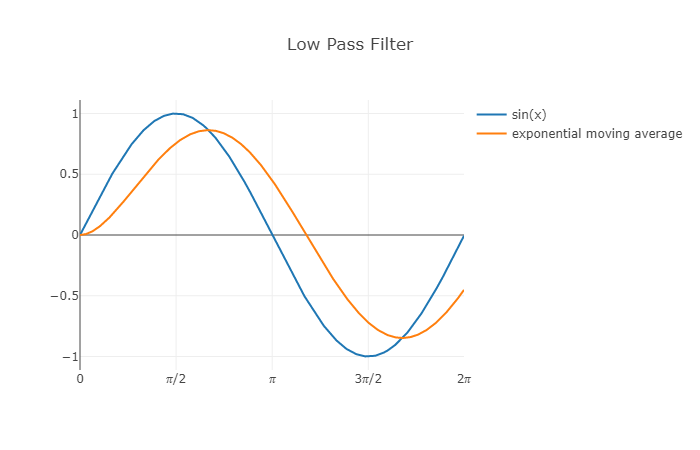
The exponential moving average is also referred to as a low pass filter. That’s because it can be used to cut off high frequency data. For example, it can be used to remove high frequency noise from audio.

In the graph below, we see the exponential moving average following the function f(x) = sin(x):

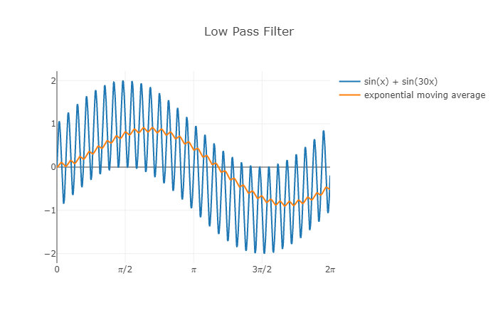
Now we add a high frequency component to the function: f(x) = sin(x) + sin(30x)

We can see that the original low frequency signal still comes through pretty clearly, but the high frequency part is significantly attenuated.

Before concluding, I will also show the formula for variance, s², that can be used to calculate the variance and standard deviation with the exponential moving average. I won’t go through the derivation steps, but again you can find the derivation in Tony Finch’s paper Incremental calculation of weighted mean and variance.

Below is a simple implementation of this logic:

class ExponentialMovingStats {
	constructor(alpha, mean) {
		this.alpha = alpha
		this.mean = !mean ? 0 : mean
		this.variance = 0
	}

	get beta() {
		return 1 - this.alpha
	}

	update(newValue) {
		const redistributedMean = this.beta * this.mean

		const meanIncrement = this.alpha * newValue

		const newMean = redistributedMean + meanIncrement

		const varianceIncrement = this.alpha * (newValue - this.mean)**2

		const newVariance = this.beta * (this.variance + varianceIncrement)

		this.mean = newMean

		this.variance = newVariance
	}

	get stdev() {
		return Math.sqrt(this.variance)
	}
}

Finally let’s compare the simple standard deviation against the exponential version with an alpha of 0.1 and the same sample data as earlier:

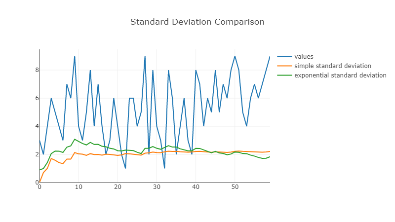
Exploring the exponential moving average introduced me to the broader world of filters. The low pass filter we’ve looked at in this article is probably one of the simplest filters. Beyond that, a whole world opens up. Filters are used in many different areas, including graphics and sound processing as well as machine learning.

Thank you to edA-qa for proofreading drafts of this article and finding several errors and issues.

References:

• Incremental calculation of weighted mean and variance, by Tony Finch
• Moving average
• Low pass filter

Related:

• Calculating a Moving Average on Streaming Data

• Calculating Standard Deviation on Streaming Data

• The Geometry of Standard Deviation