Big-O: Prime Factors and Pseudo-Polynomial Time

Most programmers have at least a passing acquaintance with big-O notation. It’s a technique that’s used to find the upper bound on running time and space requirements of algorithms as the input gets bigger.

Let’s take sorting a list as a typical example: Different algorithms will have different behaviours as the number of items to sort increases. A very simple algorithm might iterate through the list looking for the smallest item, which it brings to the front of the list. It then repeats the same process for the remainder of the list. In that case, we first go through a list of N items N times to find the smallest item, then N-1 times, N-2 times, and so on. That means we have to perform N × (N+1) / 2 comparisons. Such an algorithm is therefore in O(N²), or polynomial (quadratic to be more precise), with respect to the number of comparisons needed. In the grand scheme of things, that’s considered not so bad. However, there are better algorithms that can sort items in O(N × log N) time.

Broadly speaking the complexity of problems can be broken into 3 big categories:

1. If they’re in O(1), O(log N), O(sqrt N), O(N), or O(N × log N), algorithms are usually considered fairly tractable, which is a fancy way of saying they’re manageable.

2. Algorithms that are in polynomial complexity of at least degree 2 like O(N²), O(N³), etc. are more expensive to solve as the input gets larger. This degree of complexity is not ideal, but it’s often still okay for many kinds of real-world problems, as long as the exponent is small.

3. O(2^N) algorithms require exponential resources. That means we need to keep doubling the resources for small increases in input size. Algorithms that are exponential or worse (such as factorial), are generally considered intractable. The jump in the computational requirements happens very fast, so only small instances of such problems can be solved, even with a lot of computing power.

Sometimes people say that big-O is a measure of worst case performance. There is some nuance in the terminology though. Big-O does measure the upper bound on performance compared to the input. However, an algorithm can have a different big-O for different kinds of input. Usually best case, worst case, and average case are considered. For instance, quicksort is known to have a worst case O(N²), but typically it’s O(N × log N).

In this article, I’d like to explore something that can be tricky, namely that big-O is measured with respect to the length of the input. That means big-O can actually be different for the same algorithm, depending on how we represent the input! This may seem confusing, so let’s take a look at a concrete example.

Factoring Integers

Factoring integers to primes is a classic problem in computer science. Some widely used cryptographic algorithms, such as RSA, rely on it being a hard problem to solve as the numbers get bigger. Classical algorithms for factoring integers require exponential time in the worst case.

Factorization is not NP-complete though. If quantum computers with thousands of qbits become a reality, Shor’s algorithm can be used to factor integers in polynomial time. However, there seems to be a general consensus that even quantum computers will not make NP-complete problems tractable.

Let’s examine the most intuitive and straightforward algorithm for getting the prime factors of a number. Suppose we have an integer, say 124. How can we factor it into primes? We can start by checking if the number can be divided by 2:

124 / 2 = 62

The result is even, so let’s divide by 2 again:

62 / 2 = 31

From here we can try dividing by 3, 4, 5, etc… all the way up to 30, but all of these divisors will leave a remainder. That means 31 is also prime. It can only be divided evenly by itself or by 1. Therefore the prime factors of 124 are 2 × 2 × 31.

Only Check Factors up to the Square Root

We can make a significant optimization to this algorithm: Instead of checking all of the possible factors up to our number N itself, we only need to check numbers that are less than or equal to the square root of N: Let’s say sqrt N = S. By definition, S × S = N. Say we have an integer T that is greater than S but less than N, and T is a factor of N. That means N / T = U, where U is also a factor. Since T is greater than S, U must be less than S (otherwise T x U would be greater than N). Since U is smaller than S, we would try it as a factor before reaching S. The quotient of N / U is T. Therefore we’d already encounter T before reaching S.

To find all of the prime factors of N, that means all we need to do is try all possible factors from 2 to the square root of N inclusive. Below is a simple implementation of this algorithm in Python:

def prime_factors(n):
    results = []

    factor = 2
    while factor * factor <= n:
        (n, intermediate_results) = check_factor(n, factor)
        results += intermediate_results
        factor += 1

    if (n > 1):
        results += [n]

    return results

def check_factor(n, factor):
    results = []

    (q, r) = divmod(n, factor)
    while r == 0:
        results.append(factor)
        n = q
        (q, r) = divmod(n, factor)

    return n, results

We can further cut the running time of this algorithm in half by skipping the even numbers greater than 2, since any even factors would be extracted by checking for division by 2. While this could be significant in practice, it would not fundamentally change the complexity in terms of big-O. Big-O tends to be a coarse-grained tool that looks for the overarching pattern of growth. Constant factors and lower order terms tend to be ignored.

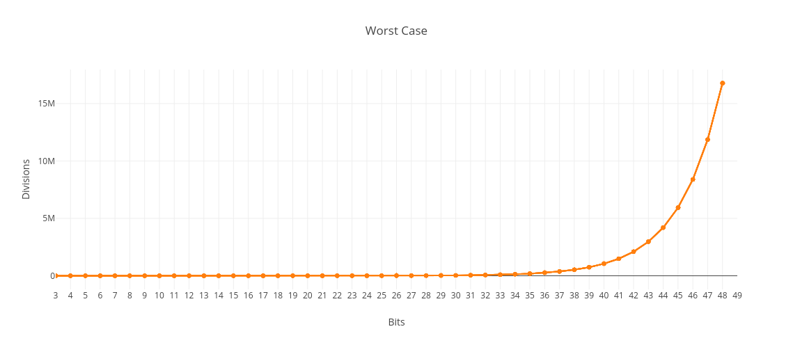
Worst Case

When we factor a number N, how many divisions do we need to perform as N increases? The worst case for our algorithm is when N is prime: Our algorithm will have to try (unsuccessfully) all of the numbers from 2 to the square root of N. Therefore our algorithm is in O (Sqrt N) for the worst case. Let’s say we try to factor the prime number 1000003. We will need to check each of the numbers from 2 to 1000, so we will perform (Sqrt N) - 1 divisions.

Input Length vs Magnitude

On the face of it, this algorithm therefore seems to be sublinear. However, there’s a key issue that’s easy to miss. The number of bits needed to encode N is log₂N. That means that the number of divisions is exponential compared to the length of the input in bits, even though it is sublinear when we compare the number of divisions to N as a magnitude. If our algorithm were in O(N), then it would be in O(2^b) where b is the number of bits in N. However, here it is in O(sqrt N). Since sqrt N requires half the number of bits in N, our algorithm turns out to be in O(2^b/2).

The graph below shows the number of divisions compared to the number of bits in N for the worst case scenario:

Instead of using decimal or binary representation, we could encode our number using unary representation, whereby 1 = 1, 2 = 11, 3 = 111, etc. In that case, our algorithm really would be in O(sqrt N). However, we’d be using much more, exponentially more, memory to store our numbers than necessary. In binary, 1000003 requires only 20 bits (11110100001001000011). In unary, it requires a million and 3 digits! In decimal, 1000003 requires 7 digits, which is even fewer than the 20 digits in binary. However, both are proportional to the log of the number, so this kind of difference is usually not very important for big-O. For example, to convert a log in base 2 to base 10, we use the equation log₁₀ N = log₂ N / log₂ 10 ≈ 1/3.32 × log₂ N. They’re directly proportional to each other.

As we increase the number of bits in N, we need exponentially more divisions to obtain the prime factors of a number. Of course the number N also increases enormously in magnitude as the number of bits goes up. That’s why this type of algorithm is sometimes referred to as being pseudo-polynomial. To see the effect of the exponential number of divisions needed, we have to keep increasing the number of bits, thus working with truly enormous numbers. The key thing to be aware of here is, I think, that the number N is the actual input, as opposed to, say, a list with N items in it.

A pseudo-polynomial-time algorithm will display ‘exponential behavior’ only when confronted with instances containing ‘exponentially large’ numbers, which might be rare for the applications we are interested in. If so, this type of algorithm might serve our purposes almost as well as a polynomial time algorithm. – Computers and Intractability, Michael R Garey and David S Johnson

Typical Case

I don’t know how to determine the big-O for the typical or average case analytically, but I tried doing some simulations to get a rough idea. We can see that the curve still looks exponential.

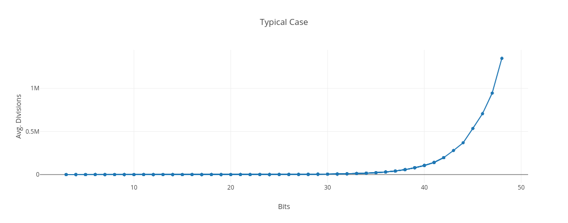
It’s clearly vastly better than the worst case though. Below is a graph of the worst case compared to this rough estimate of the typical case. I generated random numbers in the range 2^b-1 <= N < 2^b where the number of bits, b, went from 3 to 48. For each bit length, I factorized 10,000 randomly generated numbers. We can see that the number of divisions is a lot smaller for random numbers compared to primes:

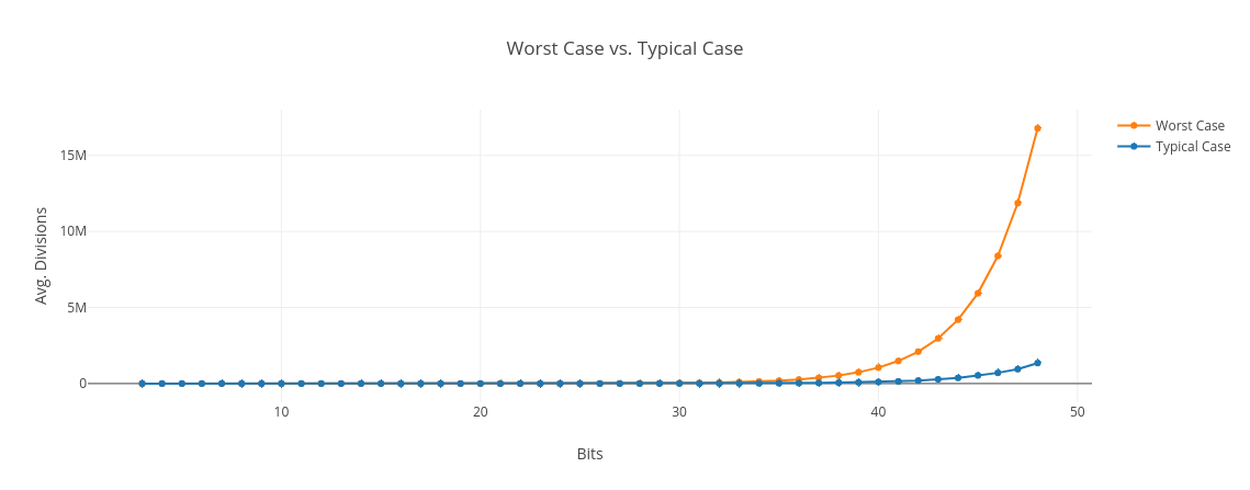
I think the reason is that, as we increase the number of bits in our numbers, the percentage of the candidate factors we need to check trends downward. It’s certainly a lot less than sqrt N. Intuitively this makes some sense to me, since we’d expect random numbers in a given range to have many more small prime factors than large ones.

These results are actually very close to what we’d expect if we used trial division with a pre-existing list of the prime factors. In that case instead of O(2^b/2), we have O(2^b/2/b × 2/ln 2). This suggests that when we select numbers at random, most of the time we do in fact just need to check a list of relatively small primes.

Also, each time we do find a prime factor, we reduce the range of factors to consider by the square root of the previous quotient. In many cases this can very rapidly cut down on the number of divisions.

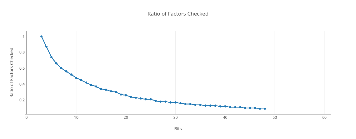
Below is the ratio of the factors that are actually checked compared with sqrt N. For 3-bit numbers, i.e., 100 (4), 101 (5), 110 (6), and 111 (7), there is only a single factor to check, 2. Since we always check this single factor, the ratio is 1, or 100%. As we get to bigger and bigger numbers, the proportion of candidate factors we have to check goes down dramatically, and trends toward zero as the number of bits goes to infinity:

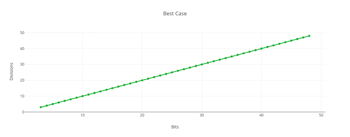
Best Case

In the best case scenario, the input is a power of 2, so all that’s needed is to keep dividing by 2. In terms of the number N, this means we only need to do log₂ N divisions. Our algorithm will be in O(log N) with respect to the magnitude of N, and in O(b) with respect to the number of bits, b, in N. While the worst case scenario is exponential, the best case scenario is linear.

Division is Not Constant

I’ve framed this article in terms of the number of divisions needed to get the prime factors of a number, as if each division only requires a constant amount of work. When dealing with numbers that can be divided directly with a machine instruction, this is a reasonable assumption. For example, if a computer has a 64-bit divide instruction, it doesn’t matter which two 64-bit numbers we’re dividing.

However, for very large numbers, that breaks down. If we divide two (huge) numbers using a simple method like long division, this becomes an O(b²) operation, where b is the number of bits in the numbers. I believe that using more advanced techniques, this can be improved, but it will remain worse than O(b × log b). However, since our prime factorization algorithm is exponential, this extra factor is probably too small to dramatically change the picture. The exponential term will tend to dominate any additional polynomial factor.

Conclusion

Even though there are better algorithms to obtain the prime factors of very large numbers, it turns out all of them are still basically exponential in the general case. Without quantum computers, there isn’t any known way to efficiently factorize numbers. RSA cryptography exploits this idea: RSA generates two very large prime numbers (each one in the thousands of bits), then multiplies them together. It relies on the intractability of finding the two prime factors of this huge resulting product.

When people are introduced to big-O, it can be easy to miss subtle points about the way that the input is encoded. I hope this article can be helpful in that regard.

The dynamic programming algorithm for the Knapsack problem is another example of a pseudo-polynomial time algorithm.

Introductions to Big-O

If you haven’t encountered the idea of big-O before, here are two popular dev.to articles that introduce the concepts of big-O and complexity:

• A coffee-break introduction to time complexity of algorithms
• Big-O Notation: Beginners Guide

References

• Trial Division