Convolutional Neural Networks: An Intuitive Primer
Neural Networks (2 Part Series)
In Neural Networks Primer, we went over the details of how to implement a basic neural network from scratch. We saw that this simple neural network, while it did not represent the state of the art in the field, could nonetheless do a very good job of recognizing hand-written digits from the mnist database. An accuracy of about 95% was quite easy to achieve.
When I learned about how such a network operates, one thing that immediately jumped out at me was that each of the neurons in the input layer was connected to all of the neurons in the next layer: As far as the network is concerned, all of the pixels start off as if they were jumbled in a random order!
In a way, this is very cool. The network learns everything on its own, not only patterns within the data, but also the very structure of the input data itself. However, this comes at a price: The number of weights and biases in such a fully connected network grows very quickly. Each mnist image has 28×28 pixels, so the input layer has 28×28, or 784 neurons. Let’s say we set up a fully connected hidden layer with 30 neurons. That means we now have 28×28×30, or 23,520 weights, plus 30 biases, for our network to keep track of. That already adds up to 23,550 parameters! Imagine the number of parameters we’d need for 4k ultra HD color images!
Introducing Convolutions
I believe this article works on its own, but it can also be considered as a supplement to chapter 6 of Neural Networks and Deep Learning, by Michael Nielsen. In that chapter, there is a general discussion of convolutional neural networks, but the details of backpropagation and chaining are left as an exercise for the reader. For the most part, these are the problems that I’ve worked through in detail in this article.
Using convolutions, it is possible to reduce the number of parameters required to train the network. We can take advantage of what we know about the structure of the input data. In the case of images for example, we know that pixels that are close to one another can be aggregated into features.
Convolution has been an important piece of the puzzle in the development of deep learning. The term deep learning sounds almost metaphysical, but its meaning is actually simple: It’s the idea of increasing the depth - the number of hidden layers - in a network. Each layer progressively extracts higher-level features from the previous layer. From wikipedia:
For example, in image processing, lower layers may identify edges, while higher layers may identify human-meaningful items such as digits/letters or faces.
How does convolution work? Let’s start with the basic idea, and we’ll get into more detail as we go along. We will start with our input data in the form of a 2-d matrix of neurons, with each input neuron representing the corresponding pixel. Next, we apply an overlay, also known as a filter, to the input data. The overlay is also a 2-d matrix that’s smaller than (or the same size as) the input matrix. We can choose the appropriate overlay size. We place the overlay over the top left-hand corner of the input data. Now we multiply the overlay with the underlay, that is, the part of the input data covered by the overlay, to produce a single value (we’ll see how this multiplication works a bit later).
We assign this value to the first neuron in a 2-d result matrix, which we’ll call a feature map. We move the overlay over to the right, and perform the same operation again, yielding another neuron for the feature map. Once we reach the end of the first row of the input in this manner, we move down and repeat the process, continuing all the way to the last overlay in the bottom right-hand corner. We can also increase how much we slide the overlay for each step. This is called the stride length. In the diagram below, the blue overlay yields the blue neuron; the red overlay produces the red neuron; and so on across the image. The green overlay is the last one in the feature map, and produces the green neuron:
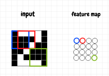
If our image is an M×N grid, and our overlay is an I×J grid (and we use a stride length of 1), then moving the overlay in this manner will produce an (M-I+1)×(J-N+1) grid. For example, if we have a 4×5 input grid, and a 2×2 overlay, the result will be a 3×4 grid. Convolution is what we call this operation of generating a new grid by moving an overlay across an input matrix.
Often convolutional layers are chained together. The raw input, such as image data, is sent to a convolutional layer that contains several feature maps. This convolutional layer may in turn be connected to another convolutional layer that further organizes the features from the previous convolutional layer. We can see in this idea the emergence of deep learning.
Feature Map Activation
In the previous section, we learned that the process of convolution is used to create a feature map. Now let’s go into a bit more detail about how this works. How do we calculate the activations for neurons in the feature map?
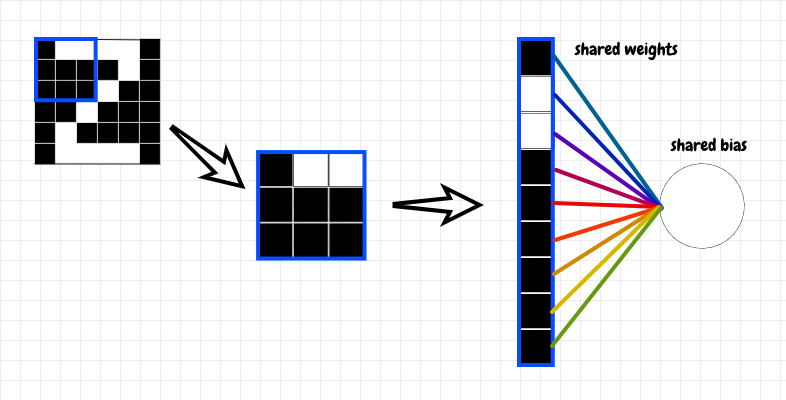
We know that an overlay, or filter, is convolved with the input data. What is this overlay? It turns out this is a matrix that represents the weights that connect each feature neuron to the underlay in the previous layer. We place an overlay of weights over the input data. We take the activation of each cell covered by the overlay and multiply it by its corresponding weight, then add these products together.
An easy way to compute this operation for a given feature neuron is to flatten the activations of the underlay into a single column and to flatten the weights filter into a single row, then perform a dot product between the weights and the activations. This multiplies each cell in the overlay with its corresponding cell in the underlay, then adds these products together. The result is a single value. This is the sense in which we multiply the overlay and the underlay as mentioned earlier.
To obtain the raw activation z for the corresponding feature neuron, we just need to add the bias to this value. Then we apply the activation function σ(z) to obtain a. Hopefully this looks familiar: To generate the activation for a single neuron in the feature map, we perform the same calculation that we used in the previous article - the difference is that we’re applying it to a small region of the input this time. This idea is shown in the diagram below:
Having performed this step to generate an activation value for the first neuron in the feature map, we can now slide the overlay of weights across the input matrix, repeating this same operation as we go along. The feature map that’s produced is the result of convolving the input matrix with the weights matrix. Actually, in math, the operation I’ve described is technically called a cross-correlation rather than a convolution. A convolution involves rotating the filter by 180° first. The two operations are very similar, and it seems the terms are often used somewhat interchangeably in machine learning. In this article, we will end up using both cross-correlation and convolution.
Note that we keep using the same matrix of weights as a filter across the entire input matrix. This is an important trick: We only maintain one bias and one set of weights that are shared among all of the neurons in a given feature map. This saves us a lot of parameters! Let’s say we have the same 28×28, or 784 input neurons and we choose a 4×4 overlay. That will produce a 25x25 feature map. This feature map will have just 16 shared weights and 1 shared bias. We will usually set up several independent feature maps in the first convolutional layer. Let’s suppose that we set up 16 feature maps in this case. That means we’ve got 17×16, or 272 parameters in this convolutional layer, far fewer than the 23,550 parameters we considered earlier for a fully connected layer.
Let’s examine a simple example: Our input layer is a 3×3 matrix, and we use a 2×2 overlay. The diagram below shows how the input matrix is cross-correlated with the the weights matrix as an overlay to produce the feature map - also a 2×2 matrix in this case:
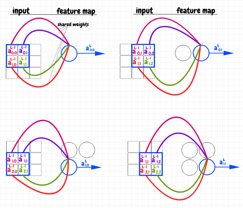
The overlay is a 2×2 matrix of weights. We start by placing this matrix over top of the activations in the top left-hand corner of the 3×3 input matrix. In the image above, each weight in the overlay matrix is represented as a colored curve pointing to the corresponding neuron in the feature map. Each activation in the underlay (the part of the input matrix covered by the overlay) is colored to match the weight it corresponds to. We multiply each activation in the underlay by its corresponding weight, then we add up these products into a single value. This value is fed into the corresponding feature neuron. We can now slide the overlay across the image, repeating this operation for each feature neuron. Again, we say that the feature map this produces is the result of cross-correlating the input data with the shared weights matrix as an overlay or filter.
The code that produces the activations for a feature map is shown below (the full code is available in the code section at the end of the article):
self.z = sp.signal.correlate2d(self.a_prev, self.w, mode="valid") + self.b
self.a = sigmoid(self.z)
What is the meaning of the shared weights and bias? The idea is that each neuron in a given feature map is looking for a feature that shows up in part of the input. What that feature actually looks like is not hard-coded into the network. The particular feature that each feature map learns is an emergent property that arises from the training of the network.
It’s important to note that, since all of the neurons in a feature map share their weights and bias, they are in a sense the same neuron. Each one is looking for the same feature across different parts of the input. This is known as translational invariance. For example, let’s say we want to recognize an image representing the letter U, as shown below:

Maybe the network will learn a vertical straight line as a single feature. It could then identify the letter U as two such features next to each other - connected by a different feature at the bottom. This is somewhat of an oversimplification, but hopefully it gets the flavour of the idea across - the vertical lines in this example would be two different neurons in the same feature map.
Keep in mind that each of the neurons in a feature map will produce the same activation if they receive the same input: If an image has the same feature in two parts of the screen, then both corresponding feature neurons will fire with exactly the same activation. We will use this intuition when we derive the calculations for backpropagation through a feature map.
For a given grid of input neurons, we likely want to train more than one feature map. Therefore, we can connect the input layer to several independent feature maps. Each feature map will have its own weights and bias, completely independent from the other feature maps in that layer. We can call such a collection of feature maps a convolutional layer.
Backpropagation through a Feature Map
Next, let’s work out how to do backpropagation through a feature map. Let’s use the same simple example of a 3×3 input matrix and a 2×2 weights filter. Since our feature map is also a 2×2 matrix, we can expect to receive ∂C/daL as a 2×2 matrix from the next layer during backpropagation.
Bias Gradient
The first step in backpropagation is to calculate ∂C/dbL. We know the following equation obtained by using the chain rule:
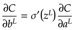
In this context, we can see that for each feature neuron, we can multiply its σ’(z) value by its ∂C/da value. This yields a 2×2 matrix that tells us the value of ∂C/db, the derivative of the cost with respect to the bias, for each feature neuron. The diagram below shows this result:
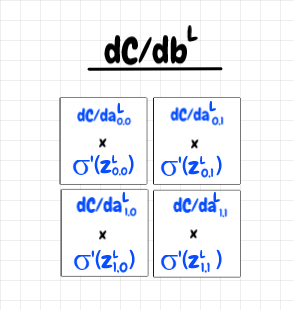
Now, all of the feature neurons share a single bias, so how should we aggregate these four values into a single value? Here, it’s helpful to recall that in a sense, all of the feature map neurons are really a single neuron.
Each neuron in the feature map receives its own small part of the previous layer as input, and produces some activation as a result. During backpropagation, ∂C/daL tells us how an adjustment to each of these activations will affect the cost function. It’s as if we only had a single neuron that received multiple consecutive training inputs, and for each of those inputs, it received a value of ∂C/daL during backpropagation. In that case, we’d adjust the bias consecutively for each training input as follows:
- b -= ∂c/db1 * step_size
- b -= ∂c/db2 * step_size
- b -= ∂c/db3 * step_size
- b -= ∂c/db4 * step_size
In fact, we can do just that. We add together the values of ∂C/db for each feature neuron. We can see that adjusting the bias using this sum produces the same result as we see in the above equations, thanks to the associativity of addition:
b -= (∂c/db1 + ∂c/db2 + ∂c/db3 + ∂c/db4) * step_size
Now that we have some intuition for this calculation, can we find a simple way to express it mathematically? In fact, we can think of this as another, very simple, cross-correlation. We have a 2×2 matrix for ∂C/daL and a 2×2 matrix for σ’(zL). Since they’re the same size, cross-correlating them together yields a single value. The cross correlation multiplies each cell in the overlay by its corresponding cell in the underlay, then adds these products together, which is the cumulative value of ∂c/dbL we want. We will also retain the four constituent values of ∂c/db for use in the subsequent backpropagation calculations.
The following line of code demonstrates this calculation (full code listing is in the code section at the end of the article):
b_gradient = sp.signal.correlate2d(sigmoid_prime(self.z), a_gradient, mode="valid")
Weight Gradient
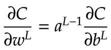
The next step in the backpropagation is to calculate ∂C/dwL. The chain rule tells us:
Can we find a way to apply this idea to our feature map in a way that makes intuitive sense? We know that each neuron in the feature map corresponds to a 2×2 portion of the previous layer’s activations. We can multiply the local value of ∂c/db for each feature neuron by each of the matching activations in the previous layer. This yields four 2×2 matrices. Each matrix represents the component of ∂C/dwL for a given neuron in the feature map. As before, we can add these all together to get the cumulative value of ∂C/dwL for this feature map. The diagram below illustrates this idea:
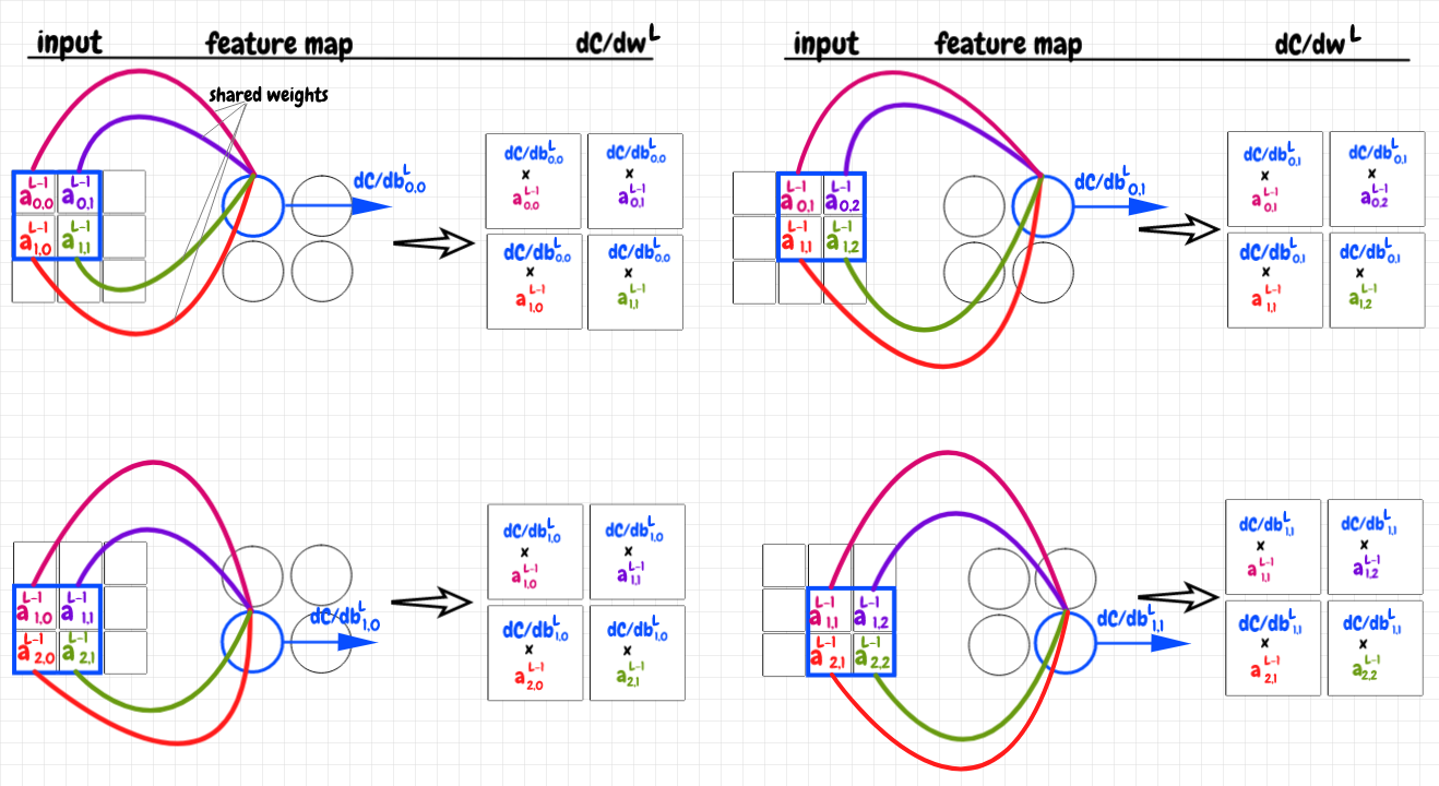
It turns out that we can concisely express this calculation as a cross-correlation as well. We can take the 3×3 matrix of activations in the previous layer and cross-correlate it with the 2×2 matrix representing the components of ∂c/db. This yields the same 2×2 matrix as the sum of the matrices in the previous diagram. The code for this logic is below (full code listing is in the code section at the end of the article):
w_gradient = sp.signal.correlate2d(self.a_prev, b_gradient_components, mode="valid")
Activation Gradient for Previous Layer
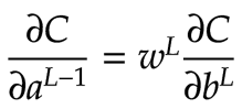
The last step in backpropagation is to calculate ∂C/daL-1. From the chain rule, we know:
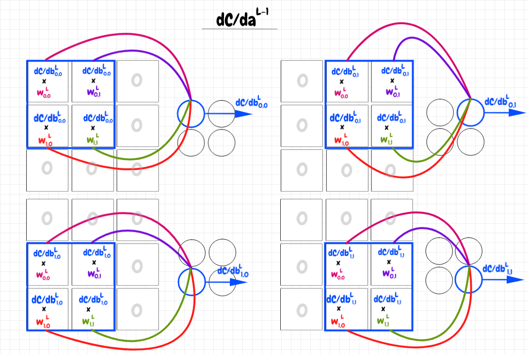
How can we make this work with our convolutional feature map? Earlier, we worked out the components of ∂C/db for each neuron in the feature map. Here, we map these values back to the overlays they correspond to in the input matrix. We multiply each component of ∂C/db by its corresponding weight for that position in the overlay. For each feature neuron, we set the parts of the input matrix that are not covered to zero. The four feature map neurons thus produce 4 3×3 matrices. These are the components of ∂C/daL-1 corresponding to each feature map neuron. Once again, to get the cumulative value, we add them together to obtain a single 3×3 matrix representing the cumulative value for ∂C/daL-1. The diagram below illustrates this process:
I found it harder to determine how to interpret this process in terms of the cross-correlation or convolution we’ve used before. After doing some research, I found out that there are several flavours of cross-correlation/convolution. For all of the calculations we’ve looked at so far, it turns out that we’ve been using valid cross-correlations. A valid convolution or cross-correlation is when the overlay stays entirely within the bounds of the larger matrix.
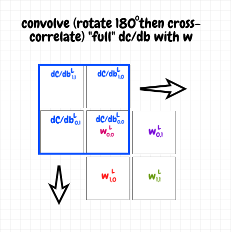
We can still use the same basic technique we’ve employed so far for this calculation as well, but we need to use a form called full convolution/cross correlation. In this variation, the overlay starts in the top left corner covering just the single cell in that corner. The rest of the overlay extends beyond the boundary of the input data. The values in that region of the overlay are treated as zeros. Otherwise the process of convolution or cross-correlation is the same. I found this link about different convolution modes helpful.
We can see that to obtain the result we want, we can apply this process using the components of the 2×2 matrix for ∂C/db as an overlay over top of the 2×2 shared weights matrix w. Since we start with the overlay covering only the single weight in the top left-hand corner, the result will be a 3×3 matrix, which is what we want for ∂C/daL-1.
In order for our calculations to match the calculations shown earlier, we need to rotate the ∂C/db filter matrix by 180° first though. That way we start with ∂C/db0,0 covering w0,0. If you follow through with this calculation, you will find that the end-result is the same as the sum of the four 3×3 matrices in the previous diagram. We’ve used the cross-correlation operation up until now. Here, since we have to rotate the filter, we are actually doing a proper convolution operation. The diagram below shows the starting position of the full convolution of ∂C/db with the weights matrix w.
The code for this is as follows (full code listing is in the code section at the end of the article):
a_prev_gradient = sp.signal.convolve2d(self.w, b_gradient_components, mode="full")
Chaining Convolutional Layers
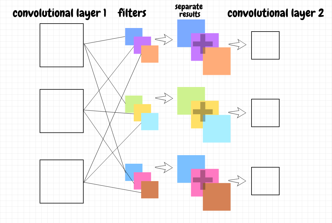
It’s common to chain together several convolutional layers within a network. How does this work? The basic idea is that the first convolutional layer has one or more feature maps. Each feature map corresponds to a single feature. Roughly speaking, each neuron in a feature map tells us whether that feature is present in the receptive field for that neuron (that is, the overlay in the previous layer for that neuron). When we send the activations from a convolutional layer to another one, we are aggregating lower-level features into higher-level ones. For example, our network might learn the shapes “◠” and “◡” as features for two feature maps in a single convolutional layer. These may be combined in a feature map in the next convolutional layer as an “O” shape.
Let’s think about how to calculate the activations. Suppose we have three feature maps in the first convolutional layer and two feature maps in the second convolutional layer. For a given feature map in the second layer, we will need a distinct weights filter for each feature map in the previous layer. In this case, that means we’ll need three filters for each feature map in the second layer. We cross-correlate each of the feature maps in the first layer with its corresponding weights filter for the feature map in the second layer. That means we generate three feature maps for the first map in the second layer and three feature maps for the second map in the second layer. We add each triple of feature maps together to produce the two feature maps we want in the second layer - we also add the bias and apply the activation function at that point. This design is similar to fully connected layers. The difference is that, instead of individual neurons, each feature map in the previous layer is connected to every feature map in the next layer.
Conceptually, we’re saying that if the right combination of the three features in the previous layer is present, then the aggregate feature that the corresponding feature map in the next layer cares about will also be present. Since there is a separate weights filter for each feature map in the previous layer, this lets us determine how the features from the previous layer need to be aggregated together for each feature in the next layer.
The diagram below illustrates how the feature maps in a given convolutional layer can be aggregated together into the next convolutional layer:
The number of filters for each feature map in the next layer matches the number of feature maps in the previous layer. The filter size determines the feature map size in the next layer.
This process can be described using 3-d matrices (see appendix B for example calculations). We combine the feature maps in the previous layer into a single 3-d matrix, like a stack of pancakes. For each feature map in the next layer, we also stack the filters into a 3-d matrix. We can cross-correlate the 3-d matrix representing the feature maps in the previous layer with the 3-d matrix representing the corresponding filters. Since both matrices have the same depth, the result will be the 2-d matrix we want for the feature map in the next layer.
To understand why we end up with a 2-d matrix, consider the case of cross-correlating or convolving two 2-d matrices in valid mode that have the same width. The result will be a 1-d matrix. For example, if we have a 7×3 matrix and we cross correlate it with a 2×3 matrix, we get a 6×1 matrix. Here it is the depth of the 3-d matrices that matches, so during cross-correlation or convolution, the values are added together depth-wise and collapsed into single values.
Backpropagation should be an application of all of the principles we’ve worked out so far:
- We use our usual method to obtain a 2-d matrix representing the components of ∂C/db for a given feature map in the next layer.
- To calculate the gradient for the filters, ∂C/dw, for that next-layer feature map, we cross-correlate the 3-d feature map activation matrix from the previous layer with our 2-d ∂C/db matrix representing the bias gradient components. This gives us a 3-d matrix for ∂C/dw for the current feature map in the next layer - each slice corresponds to the weights for one of the feature maps in the previous layer.
- For ∂C/daL-1, we convolve our 3-d weight matrix, w, with our 2-d ∂C/db matrix for a given feature map in the next layer. This gives us a 3-d matrix for ∂C/daL-1 that represents the derivative of the cost with respect to the activations of each feature map in the previous layer (corresponding to our current feature map in the next layer). We repeat this calculation for each feature map in the next layer and add together the resulting matrices. Each slice of this final matrix represents the value of ∂C/da for the corresponding feature map in the previous layer.
When we correlate or convolve what we may think of in conceptual terms as a 2-d matrix with a 3-d matrix, we need to wrap the 2-d matrix in an extra set of brackets - technically these operations require both sides to have the same dimensionality.
Max Pooling
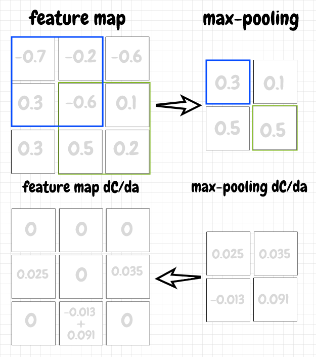
Another technique that’s sometimes used with convolutional layers is max pooling. The idea is pretty simple: We move an overlay across a feature map in a way that’s similar to convolution. However, each neuron in a max pooling mapping just takes the neuron from the corresponding overlay that has the highest activation and passes that activation to the next layer. This clearly further reduces the number of parameters, so that’s one benefit of this technique. I believe, by abstracting the input, it can also help to avoid the overfitting problem, an issue that comes up frequently in machine learning.
The backpropagation for max pooling is straightforward. For a neuron in a max pooling map, we simply pass back the value of ∂C/da to the neuron with the max activation in the corresponding overlay from the previous layer. The other gradient values in the overlay are set to 0, since those neurons did not pass along their activations, and therefore did not contribute to the cost. The diagram below shows the forward and back propagation steps for a max pooling map:
Discussion
Convolutional neural networks, or CNNs, represent a significant practical advance in the capabilities of neural networks. Such networks can achieve better accurancy as well as improved learning speed. In Michael Nielsen’s Neural Networks and Deep Learning, he combines a CNN with some other techniques to achieve over 99% accuracy recognizing the mnist digits! That’s a significant improvement over the 95% achieved using a fully connected network.
However, it is worth noting that CNNs are not a panacea. For example, while CNNs do a good job of handling translational invariance across the receptive field, they don’t handle rotation.
In this article, I’ve endeavoured to highlight the key differences between convolutional and fully connected networks. To do so, I’ve tried to keep as much logic as possible the same as in the previous article. For example, we continue to use the sigmoid activation function in this article. In practice, this is rarely the case. In deep learning, in addition to convolution, we usually see the use of some other techniques:
- The quadratic cost function is replaced with something else, e.g. a cross-entropy cost function
- Instead of sigmoid, different activation functions are used like ReLU, Softmax, etc.
- Regularization is applied to network weights in order to reduce overfitting
Code
Below I’ve implemented several classes for demonstration purposes. There’s a FeatureMap that implements forward and backpropagation for a single feature. Several such feature maps would normally be used to put together a single convolutional layer. There’s also a MaxPoolingMap which implements max pooling from a feature map. Lastly, there’s a FullyConnectedLayer, which implements the logic discussed in the previous article. In CNNs, there are usually several convolutional layers and then a fully connected layer as the last hidden layer. This fully connected layer effectively aggregates all of the feature-building stages that precede it before sending its activations to the output layer (it occurs to me that we can also implement this as a convolutional layer where each feature map is a 1×1 matrix).
import numpy as np
import scipy as sp
from scipy import signal

class FeatureMap:
    def __init__(self, a_prev, overlay_shape):
        # 2d matrix representing input from previous layer
        self.a_prev = a_prev

        # shared weights and bias for this layer
        self.w = np.random.randn(*overlay_shape)
        self.b = np.random.randn(1,1)

    def feed_forward(self):
        self.z = sp.signal.correlate2d(self.a_prev, self.w, mode="valid") + self.b
        self.a = sigmoid(self.z)

        return self.a

    def propagate_backward(self, a_gradient, step_size):
        b_gradient_components = dc_db(self.z, a_gradient)

        b_gradient = sp.signal.correlate2d(sigmoid_prime(self.z), a_gradient, mode="valid")
        w_gradient = sp.signal.correlate2d(self.a_prev, b_gradient_components, mode="valid")
        a_prev_gradient = sp.signal.convolve2d(self.w, b_gradient_components, mode="full")

        self.b -= b_gradient * step_size
        self.w -= w_gradient * step_size
        self.a_prev_gradient = a_prev_gradient

        return self.a_prev_gradient

class MaxPoolingMap:
    def __init__(self, a_prev, overlay_shape):
        self.a_prev = a_prev
        self.overlay_shape = overlay_shape

    def feed_forward(self):
        self.max_values, self.max_positions = max_values_and_positions(
            self.a_prev, self.overlay_shape)

        return self.max_values

    def propagate_backward(self, a_gradient):
        a_prev_gradient = np.zeros(self.a_prev.shape)

        rows, cols = self.max_values.shape
        for r in xrange(rows):
            for c in xrange(cols):
                max_position = self.max_positions[r][c]
                a_prev_gradient[max_position] += a_gradient[r][c]

        self.a_prev_gradient = a_prev_gradient

        return self.a_prev_gradient

class FullyConnectedLayer:
    def __init__(self, a_prev, num_neurons):
        self.a_prev = a_prev
        self.num_neurons = num_neurons

        self.w = np.random.randn(num_neurons, a_prev.size)
        self.b = np.random.randn(num_neurons,1)

    def feed_forward(self):
        a_prev = as_col(self.a_prev)

        self.z = raw_activation(self.w, a_prev, self.b)
        self.a = sigmoid(self.z)

        return self.a

    def propagate_backward(self, a_gradient, step_size):
        b_gradient = dc_db(self.z, a_gradient)

        a_prev = as_col(self.a_prev)
        weights_gradient = dc_dw(a_prev, b_gradient)

        a_prev_gradient = dc_da_prev(self.w, b_gradient)
        self.a_prev_gradient = a_prev_gradient.reshape(self.a_prev.shape)

        self.b -= b_gradient * step_size
        self.w -= weights_gradient * step_size

        return self.a_prev_gradient

# utility functions

def sigmoid(z):
    return 1.0/(1.0+np.exp(-z))

def sigmoid_prime(z):
    return sigmoid(z)*(1-sigmoid(z))

def dc_db(z, dc_da):
    return sigmoid_prime(z) * dc_da

def get_feature_map_shape(input_data_shape, overlay_shape):
    input_num_rows, input_num_cols = input_data_shape
    overlay_num_rows, overlay_num_cols = overlay_shape
    num_offsets_for_row = input_num_rows-overlay_num_rows+1
    num_offsets_for_col = input_num_cols-overlay_num_cols+1

    return (num_offsets_for_row, num_offsets_for_col)

def get_max_value_position(matrix):
    max_value_index = matrix.argmax()
    return np.unravel_index(max_value_index, matrix.shape)

def max_values_and_positions(a_prev, overlay_shape):
    feature_map_shape = get_feature_map_shape(a_prev.shape, overlay_shape)
    max_values = np.zeros(feature_map_shape)
    max_positions = np.zeros(feature_map_shape, dtype=object)

    overlay_num_rows, overlay_num_cols = overlay_shape
    feature_map_rows, feature_map_cols = feature_map_shape
    for r in xrange(feature_map_rows):
        for c in xrange(feature_map_cols):
            overlay = a_prev[r:r+overlay_num_rows, c:c+overlay_num_cols]
            max_value = np.amax(overlay)
            max_value_overlay_row, max_value_overlay_col = get_max_value_position(overlay)
            max_value_row = r+max_value_overlay_row
            max_value_col = c+max_value_overlay_col

            max_values[r][c] = max_value
            max_positions[r][c] = (max_value_row, max_value_col)

    return (max_values, max_positions)

def raw_activation(w, a, b):
    return np.dot(w,a) + b

def dc_dw(a_prev, dc_db):
    return np.dot(dc_db, a_prev.transpose())

def dc_da_prev(w, dc_db):
    return np.dot(w.transpose(), dc_db)

def as_col(matrix):
    return matrix.reshape(matrix.size, 1)

input_data = np.arange(20).reshape(4,5) # 4x5 array
overlay_shape = (2, 2)
cl = FeatureMap(input_data, overlay_shape)
cl.feed_forward()
fl_shape = get_feature_map_shape(input_data.shape, overlay_shape)
cl.propagate_backward(np.random.randn(*fl_shape), 0.1)

max_pool_input_data = np.array([[8,0,11,1,6],[10,2,4,14,17],[5,16,19,15,7],[12,13,9,18,3]])
mpl = MaxPoolingMap(max_pool_input_data, overlay_shape)
mpl.feed_forward()
fl_shape = get_feature_map_shape(max_pool_input_data.shape, overlay_shape)
mpl.propagate_backward(np.random.randn(*fl_shape))

fcl = FullyConnectedLayer(input_data, 10)
fcl.feed_forward()
fcl.propagate_backward(as_col(np.random.randn(10)), 0.1)
Appendix A: Valid vs. Full Mode
The python REPL code below shows how to use cross-correlation and convolution using valid and full modes. Note how convolute2d produces the same result as correlate2d with a filter that’s rotated by 180°.
>>> import numpy as np
>>> import scipy as sp
>>> from scipy import signal
>>> values = np.array([[1,2,3],[4,5,6],[7,8,9]])
>>> values
array([[1, 2, 3],
       [4, 5, 6],
       [7, 8, 9]])
>>> f = np.array([[10,20],[30,40]])
>>> f
array([[10, 20],
       [30, 40]])
>>> sp.signal.correlate2d(values,f,mode="valid")
array([[370, 470],
       [670, 770]])
>>> sp.signal.convolve2d(values,f,mode="valid")
array([[230, 330],
       [530, 630]])
>>> f_rot180 = np.rot90(np.rot90(f))
>>> f_rot180
array([[40, 30],
       [20, 10]])
>>> sp.signal.correlate2d(values,f_rot180,mode="valid")
array([[230, 330],
       [530, 630]])
>>> sp.signal.correlate2d(values,f,mode="full")
array([[ 40, 110, 180,  90],
       [180, 370, 470, 210],
       [360, 670, 770, 330],
       [140, 230, 260,  90]])
>>> sp.signal.convolve2d(values,f,mode="full")
array([[ 10,  40,  70,  60],
       [ 70, 230, 330, 240],
       [190, 530, 630, 420],
       [210, 520, 590, 360]])
>>> sp.signal.correlate2d(values,f_rot180,mode="full")
array([[ 10,  40,  70,  60],
       [ 70, 230, 330, 240],
       [190, 530, 630, 420],
       [210, 520, 590, 360]])
Appendix B: Summing 2-D vs. 3-D Stack:
The REPL code below shows that performing separate 2-d cross-correlations and adding them together produces the same result as stacking the inputs and the filters, then cross correlating these two 3-d matrices together:
>>> feature_map1 = np.array([[1,2,3],[4,5,6],[7,8,9]])
>>> feature_map2 = np.array([[9,8,7],[6,5,4],[3,2,1]])
>>> filter1 = np.array([[1,2],[3,4]])
>>> filter2 = np.array([[5,6],[7,8]])
>>> feature_map1
array([[1, 2, 3],
       [4, 5, 6],
       [7, 8, 9]])
>>> feature_map2
array([[9, 8, 7],
       [6, 5, 4],
       [3, 2, 1]])
>>> filter1
array([[1, 2],
       [3, 4]])
>>> filter2
array([[5, 6],
       [7, 8]])
>>> result1 = sp.signal.correlate2d(feature_map1, filter1, mode="valid")
>>> result1
array([[37, 47],
       [67, 77]])
>>> result2 = sp.signal.correlate2d(feature_map2, filter2, mode="valid")
>>> result2
array([[175, 149],
       [ 97,  71]])
>>> sum_of_results = result1 + result2
>>> sum_of_results
array([[212, 196],
       [164, 148]])
>>> feature_maps_stacked = np.array([feature_map1, feature_map2])
>>> feature_maps_stacked
array([[[1, 2, 3],
        [4, 5, 6],
        [7, 8, 9]],

       [[9, 8, 7],
        [6, 5, 4],
        [3, 2, 1]]])
>>> filters_stacked = np.array([filter1, filter2])
>>> filters_stacked
array([[[1, 2],
        [3, 4]],

       [[5, 6],
        [7, 8]]])
>>> stacked_results = signal.sp.correlate(feature_maps_stacked, filters_stacked, mode="valid")
>>> stacked_results.reshape(2,2) # same as sum_of_results
array([[212, 196],
        [164, 148]])