The Geometry of Standard Deviation

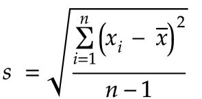
I recently needed to look up the formula for standard deviation. It struck me that the formula looks a bit mysterious, with its squares and square roots. Here’s the basic formula for the standard deviation of a sample of data:

We subtract each measurement from the mean (this is often just called the ‘average’) and take the square. We add all of these squares up, and divide by n-1. Finally we take the square root. What’s going on here?

Looking at this formula for the first time in a while, it occurred to me that the numerator looks a lot like the distance in the Pythagorean theorem. The diagram below shows the distance d between 2 points, p1 and p2:

According to the Pythagorean theorem, this distance is:

It’s similar, right? We have a square root. Inside the square root we sum up some values. Each item in the sum is the square of a difference. It’s the same basic operation as in the numerator for our standard deviation.

Let’s explore this with a very basic specific case: Suppose we have two values in a sample of data, say, x₁ = 2.5 and x₂ = 1.5. The mean is (2.5 + 1.5)/2 = 2.

Now, let’s calculate the distance between two points: The first point consists of both sampled measurements. The first measurement is on the x-axis, and the second measurement is on the y-axis. We’ll call this point V, since it represents the sampled values. V = (x₁, x₂) = (2.5, 1.5).

The measurement x₁ is on the x-axis, but the measurement x₂ is on the y-axis, so I am departing now from the convention that x refers to the x axis. It’s just a variable. We could call these values v₁, v₂ as well.

The second point, which we’ll call M for the mean, consists of the mean, x̄, on both axes. M = (x̄, x̄) = (2, 2).

We can see that the distance between V and M is:

Now let’s see if we can connect this distance between two points with the formula for standard deviation.

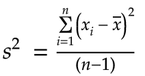
The square of a sample’s standard deviation is called the variance and is denoted s²:

Let’s multiply the variance by n-1:

Now let’s take the square root:

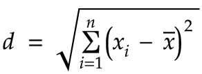
Let’s define this value we’ve just derived as d:

We can now see that the distance that we computed earlier, 0.71, is in fact this value d!

With just some minor algebra, we can show that the standard deviation is closely related to this distance:

As we can see, we can get the standard deviation by dividing d by √(n-1). In this particular case, √(n-1) is just 1. Thus we can say the standard deviation is 0.71!

This worked well for a case where we had 2 measurements in our sample, but what do we do if we have (as is usually the case) more than 2 data points? If we had 3 measurements, then the our point V would have 3 dimensions, V = (x₁, x₂, x₃). Our point M would also have 3 dimensions, M = (x̄, x̄, x̄).

The cool part is that we can extend the number of dimensions arbitrarily for each of the measurements in our sample. V = (x₁, x₂, x₃, … x_n), and M = (x̄, x̄, x̄, … x̄).

M will always be a point along the diagonal since it will have the same value, x̄, on every axis.

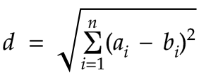
The Pythagorean theorem holds for any number of dimensions. In fact, the formula for the distance between 2 points a and b in n dimensions should hopefully look familiar:

Let’s compare with d that we defined earlier:

Using this idea of distance is probably not useful for visualizing the standard deviation for a sample that’s larger than 3 data points (i.e. 3 dimensions) but I think it’s helpful in building a greater conceptual understanding of what the standard deviation represents.

With standard deviation, we’re trying to measure the ‘spread’ or ‘variability’ of some data. If all the values in a sample are the same, then of course the distance between the points V and M will be 0. That means the standard deviation will also be 0. The more variable the data is, the farther away the point V will be from the point M.

When we divide by √(n-1), we are normalizing this distance, essentially averaging out the contribution of each value in the sample to the distance from V to M.

This idea of geometry in n dimensions may be a bit intimidating. I think here it makes intuitive sense that each piece of data needs to be on its own axis though: We want each value to contribute to the variability independently. We wouldn’t want a value of +4 to cancel out a value of -4 when determining the variance or the standard deviation.

If it was new to you, I hope this geometric perspective has helped to build intuition for what standard deviation really is rather than just being a formula to memorize. Thank you for reading!

If we are calculating the standard deviation in a case where we’ve included all of the possible data, then we actually divide by n to calculate the variance. This may work, for example, when calculating the statistics for all of the grades on an exam, or when calculating the statistics for a medical trial.

In most cases though, we take a sample that is just a fraction of the total data. In that case, we usually divide by something like n-1. Why we do this is a bit of a mystery of its own. For more information, check out Bessel’s Correction and Degrees of Freedom.

Related:

• Calculating a Moving Average on Streaming Data
• Calculating Standard Deviation on Streaming Data
• Exponential Moving Average on Streaming Data