Tic-Tac-Toe with Tabular Q-Learning
Tic-Tac-Toe (4 Part Series)
2. Tic-Tac-Toe with Tabular Q-Learning
In the last article, we implemented a tic-tac-toe solver using minimax. Minimax is great, but it does have a couple of issues. First of all, while it doesn’t make mistakes, it also doesn’t take full advantage of patterns that might be found in the opponent’s moves. Second, minimax is often not practical. Historically, in the case of of chess, variations that bolted various heuristics on top of minimax were actually pretty successful. These strategies were good enough to build chess engines that could defeat even the best human players in the world. For go, the situation was less satisfactory: Prior to DeepMind’s breakthrough with AlphaGo in 2015, the best AIs used monte-carlo tree search (MCTS), a close cousin of minimax. Such AIs managed to rate as fairly strong amateur players, but they were not anywhere near beating a professional human player.
DeepMind revolutionized the world of games like chess and go (and to an extent the field of machine learning in general) with the application of deep neural networks. Not only are these deep learning implementations superior to anything that has come before in terms of strength, they also display a much more original and flexible approach to the way they play, which has completely upended a lot of the traditional theory of games like chess and go. This success of deep learning is remarkable - and also kind of surprising to me as I learn more about the underlying dynamics. For example, with go, I’m still puzzled that deep learning can be so exquisitely sensitive to very small differences in game state.
In this article we will implement reinforcement learning using tabular Q-learning for tic-tac-toe, a step toward applying such ideas to neural networks. Like training a pet, reinforcement learning is about providing incentives to gradually shape the desired behaviour. The basic idea of tabular Q-learning is simple: We create a table consisting of all possible states on one axis and all possible actions on another axis. Each cell in this table has a Q-value. The Q-value tells us whether it is a good idea or not to take the corresponding action from the current state. A high Q-value is good and a low Q-value is bad. The diagram below shows the basic layout of a Q-table:
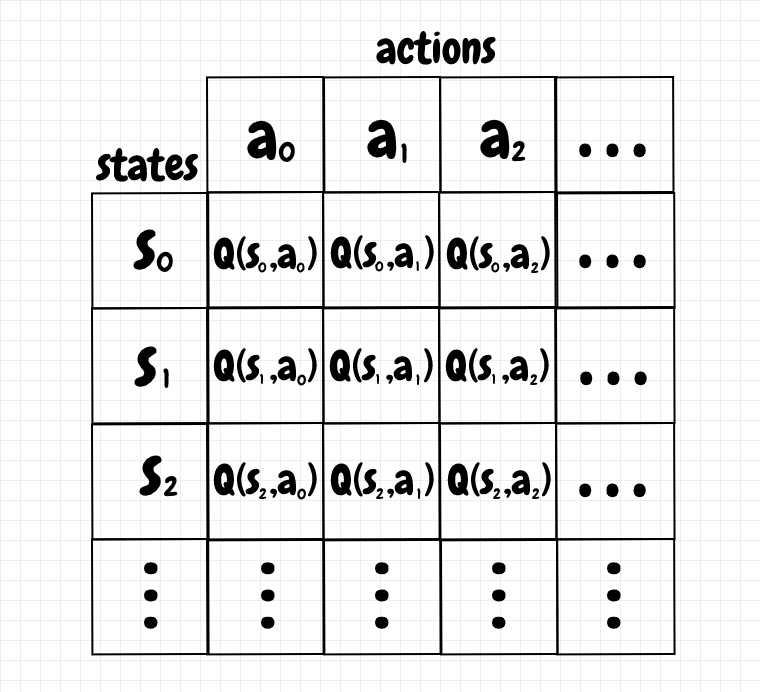
During reinforcement learning, our agent moves from one state to another by taking actions. The transition from one state to another produced by a given action may also incur a reward. Rewards increase the associated Q-values. We can also assign a negative reward as a punishment for an action, which reduces the Q-value, and therefore discourages taking that action from that particular state in the future. By the end of the training, for a given state, we pick the action that corresponds to the highest Q-value.
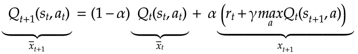
How do we update the values of our state-action pairs in the Q-table? Q-learning defines a function that allows us to iteratively update the Q-values in the table. If we’re in a given state, and we take a particular action, the equation below shows how we update the corresponding Q-value:

Before getting into detail, note that this equation is an exponential moving average, which I’ve written about in a previous article. Below is the formula for the exponential moving average:
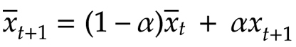
In the case of the exponential moving average, we receive a new value xt+1 and apply 𝛼, a value between 0 and 1 to it. 𝛼 defines how strongly a new value will affect the average. The closer this value is to 1, the more closely the exponential moving average will just track the incoming data. We adjust the current average (prior to the update) by 1-𝛼, and the new average becomes the sum of these two terms. For instance, if 𝛼 is 0.1, a new value will contribute to 10% of the updated average, and all of the previous values combined will contribute 90%. With the function that updates the Q-value, it’s the same idea: We receive an update for our Q-value for a given state/action pair and apply 𝛼 to it. We then apply 1-𝛼 to the existing Q-value. The new Q-value becomes the sum of these two values. In the diagram below, we can see how the terms in the Q-value update function correspond to the terms in the exponential moving average:
For the case of tic-tac-toe, it seems to me that we don’t actually need to use a moving average - we could probably just add the new values to the current total. I think it makes sense to choose this approach when there are large number of updates: The exponential moving average is more numerically stable. Also, if we’re working within a domain where the the value for a state/action pair can change over time, this approach also lets us value recent information over older information.
Let’s explore the terms in the update function in a bit more detail. On the left, we assign a new Q-value for a given state/action pair. If we know the Q-value at time t, the new Q-value corresponds to time t+1. On the right, we take the current Q-value for that state/action pair at time t, and multiply it by 1-𝛼, and we add it to the incoming update for the Q-value, scaled by 𝛼, shown below:
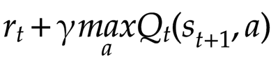
- When we take a given action from a particular state, we go to the next state, st+1. The transition into this new state may earn us a reward. That’s the value of rt in the above equation.
- We also look at the Q-values for all possible actions from the new state, st+1, that we enter after we take our action at. We pick the maximum Q-value for this next state and use it to update our current Q-value. The idea is that our Q-value will also depend on the best Q-value we can get from the following state (which depends on the state after that, and so on).
- We can adjust the maximum Q-value from the next state by a discount factor 𝛾 (gamma), between 0 and 1. If 𝛾 is low, that means we will value immediate rewards, denoted by rt, over future rewards, as characterized by the Q-values of subsequent states.
In summary, we update the Q-value for a given state/action pair by using an exponential moving average. The incoming update is obtained by balancing the reward obtained in the current state and the maximum Q-value from next state.
Tic-Tac-Toe
To train a tabular Q-value agent to play tic-tac-toe, we’ll use board positions as the states, and the moves played as the actions. We’ll define a Q-value for each such state/action pair we encounter. When we reach an end-of-game state, the result of the game is the reward assigned to the move that led to that result. We can then work our way back through the history of the game and update the Q-value for each action taken by the Q-table agent during the game. The diagram below shows a sample training game where all of the Q-values start at 0. For illustration, we’ll use a high 𝛼 of 0.9:
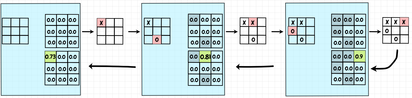
X is the Q-table agent and it’s being trained against an O player that just plays randomly. Since X’s last move leads to a win, we give that action a reward of +1. The Q-value becomes 0 + 𝛼 * 1, or 0.9. We can now update the previous action in the game history. Since this move doesn’t end the game, there is no direct reward. Also, since rewards are only assigned for the last action taken by the Q-table agent, I believe we can set the discount factor, 𝛾, to 1 - that is, there is no need to further discount future rewards. The maximum Q-value for the next state is 0.9, so we update our Q-value to 0 + 𝛼 * 0.9, or 0.81. Going one state further back in the history, we reach the starting position. The maximum Q-value for the next state is 0.81, so our new Q-value for the first move becomes 0 + 𝛼 * 0.81, or 0.729 (rounded to 0.73 in the diagram). To train our Q-table agent, we repeat this process with many training games.
Note that for a Q-learning agent, the next state it sees will be the state of the board after the opponent’s response (or an end-of-game state). Since it doesn’t control the opponent, the Q-table player considers the result of its move to be whatever happens after the opponent responds. In this sense, the “next state” isn’t the state that follows the Q-table agent’s move - it’s the state that results from the opponent’s follow-up move.
Epsilon-Greedy
If we just update the Q-values by using the existing values in the Q-table, this can create a feedback cycle that reinforces Q-values that are already high. To mitigate this problem, one approach is to use an epsilon-greedy strategy (aka ε-greedy). The idea is simple: We set an ε value between 0 and 1. Before choosing an action, we generate a random number, also between 0 and 1 (with a uniform probability distribution). If the random number is less than ε, we choose a random move. Otherwise we choose a move using the Q-table. In other words, we choose a random move with probability ε, and we use a move from the Q-table with probability 1-ε: Choosing a random move is called exploration, whereas using the Q-table values is called exploitation.
Choosing a high value for ε, say 0.9, means we will play randomly 90% of the time. In the example code, we start with a high ε value and gradually decrease it to 0. That way, we do more exploration early on, trying out all kinds of different ideas, and then we increasingly rely on the Q-table values later on. By the end of the training, we use the Q-table exclusively.
Double-Q Learning
Q-learning with a single table can apparently cause an over-estimation of Q-values. This appears to happen because, when we update the Q-value for a given state/action pair, we are using the same Q-table to obtain the maximum Q-value for the next state - as we saw in our tic-tac-toe example calculation earlier. To loosen this coupling, double Q-learning introduces a pair of Q-tables. If we are updating a Q-value for Q-table a, then we obtain the maximum Q-value for the next state from Q-table b. Conversely, if we are updating Q-table b, we get the maximum Q-value for the next state from Q-table a. For reference, see the papers Double Q-learning and Deep Reinforcement Learning with Double Q-learning. I’ve adapted the pseudo-code from the paper on Double Q-learning below:
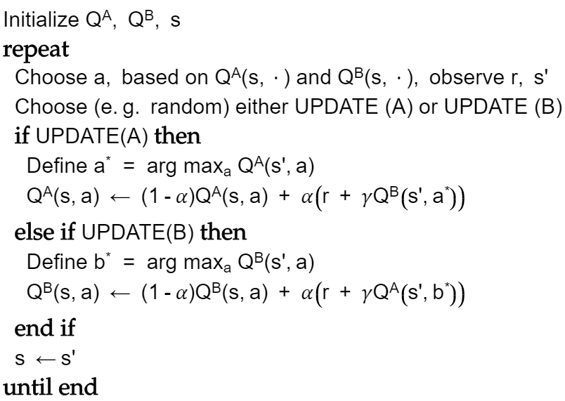
The pseudo code above does not stipulate how the next action is chosen. Here’s what I do in my tic-tac-toe code (from qtable.py):
def choose_move_index(q_tables, board, epsilon):
    if epsilon > 0:
        random_value_from_0_to_1 = np.random.uniform()
        if random_value_from_0_to_1 < epsilon:
            return board.get_random_valid_move_index()

    move_q_value_pairs = get_move_average_q_value_pairs(q_tables, board)

    return max(move_q_value_pairs, key=lambda pair: pair[1])[0]
We use epsilon-greedy to decide whether to make a random move. If the decision is not to play randomly, and we are using double Q-learning, then we get the Q-values for this position from both Q-tables and average them.
We can also see from the pseudo code that we obtain the action (arg) of the maximum Q-value from the current table, but then we actually use the Q-value corresponding to this action from the other Q-table. Below is the code that performs Q-table updates for the tic-tac-toe agent (from qtable.py):
def update_training_gameover(q_tables, move_history, q_table_player, board,
                             learning_rate, discount_factor):
    game_result_reward = get_game_result_value(q_table_player, board)

    # move history is in reverse-chronological order - last to first
    next_position, move_index = move_history[0]
    for q_table in q_tables:
        current_q_value = q_table.get_q_value(next_position, move_index)
        new_q_value = (((1 - learning_rate) * current_q_value)
                       + (learning_rate * discount_factor * game_result_reward))
        q_table.update_q_value(next_position, move_index, new_q_value)

    for (position, move_index) in list(move_history)[1:]:
        current_q_table, next_q_table = get_shuffled_q_tables(q_tables)

        max_next_move_index, _ = current_q_table.get_move_index_and_max_q_value(
            next_position)

        max_next_q_value = next_q_table.get_q_value(next_position,
                                                    max_next_move_index)

        current_q_value = current_q_table.get_q_value(position, move_index)
        new_q_value = (((1 - learning_rate) * current_q_value)
                       + (learning_rate * discount_factor * max_next_q_value))
        current_q_table.update_q_value(position, move_index, new_q_value)

        next_position = position
For each position in a given game history, we start with the last move played by the Q-table agent and work our way backward. Since we know the result of the game for the last position, we use that to update the Q-value for both Q-tables. From there, we randomly select a Q-table to update, and we get a Q-value for the next state in the game from its companion Q-table. The code above is generic - if there is just one Q-table, it will keep re-using that single table.
According to the papers mentioned above, double Q-learning produces results that are more stable and converge to higher scores faster. However, in implementing this for my tic-tac-toe player, I didn’t find an improvement. In fact, the results seem to be better using a single Q-table.
Results
Even with this simple case study of tic-tac-toe, there is already a fair amount of complexity involved in tuning this tabular Q-learning algorithm. We have to choose reward values for wins, draws, and losses. Choosing +1 for a win, 0 for a draw, and -1 for a loss seems to work. We also need to choose default starting Q-values. I did not play around with this too much, but just initializing them to a neutral 0 seems okay.
Then we have to select a value for 𝛼 (the learning rate), 𝛾 (the discount factor), and ε (for epsilon-greedy). Lastly, we have to choose what kind of opponent to train our Q-learning agent against, and how many training games to use. I’ve managed to obtain what I hope are reasonable results using 0.4 for 𝛼, and 1 for 𝛾 (since we only receive rewards for end-of-game states). I also start the agent with aggressive exploration using an ε of 0.7. This value is reduced by 0.1 for every 10% of training games. After 7000 training games against an opponent that just chooses moves at random, these parameters usually produce results that generalize well to different opponents, shown below:
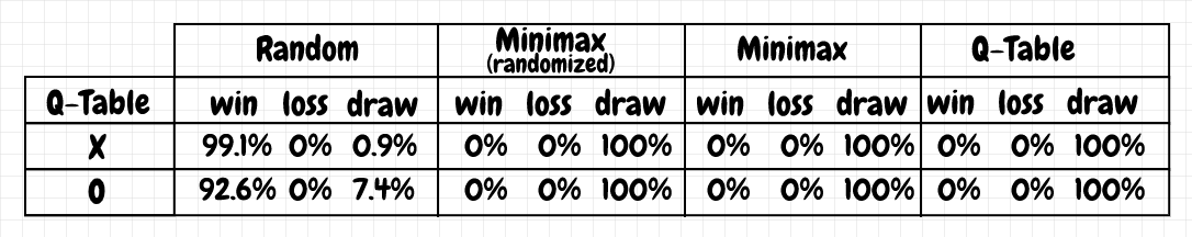
These results are obtained from 1,000 games played against each of several opponents. The opponents consist of 1) a player that makes random moves; 2) a randomized minimax player (where a random move is chosen from several “best moves” of equal value); 3) a deterministic minimax player (where the first “best move” is chosen); 4) another Q-table agent. The results above are actually even better than for minimax: The Q-table player doesn’t makes mistakes, just like minimax, but it has more wins against a random player than minimax does. I was surprised that training against an agent that plays randomly was good enough for the Q-table player to make no mistakes against both randomized and deterministic minimax opponents.
While these results look good, I’ve noticed that occasionally, a training run using this configuration can yield poor results as O against the randomized minimax player. The Q-table player suddenly loses about 40% of the games (and manages a draw for the rest). I know that DeepMind have applied Q-learning to neural networks - they’ve called this DQN - so this apparent tendency to overfit is something that I hope to look into more.
Update: After writing the article about Tic-Tac-Toe with MCTS, it occurred to me to try increasing the reward for a draw for tabular Q-learning (since only a draw is possible with perfect play for both sides). I wound up ratcheting the reward for a draw all the way up from 0.0 to 1.0 (same as a win). That appears to have fixed the problem with inconsistency from one training run to another. It does seem to reduce the winning percentage against random though, down to about 95% as X and around 70% as O (the remaining games are a draw).
Below are the results from training the Q-table player against a randomized minimax player, with all other parameters held the same:
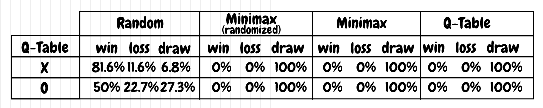
These results are not as good. This agent doesn’t win as many games against the player that makes random moves. More importantly it consistently makes mistakes - that is, it loses quite a few games against a player that makes random moves. It seems especially vulnerable when it’s playing as O, winning only 50%, and losing 22.7% of its games. The same agent trained against only the random moves player, wins 92.6% of those games. I was surprised that these results turned out to be noticeably worse overall compared to an agent that trained against a “dumber” opponent. I think the reason may be that the agent sees fewer distinct states, even with the epsilon-greedy strategy enabled. Here, the Q-table only had 355 board positions in it after training (out of 627 total board positions, excluding end-of-game states, and taking symmetry into account).
Code
The full code is available on github (qtable.py):
Experimenting with different techniques for playing tic-tac-toe
Demo project for different approaches for playing tic-tac-toe.
Code requires python 3, numpy, and pytest. For the neural network/dqn implementation (qneural.py), pytorch is required.
Create virtual environment using pipenv:
Install using pipenv:
pipenv shellpipenv install --dev
Set PYTHONPATH to main project directory:
- In windows, run
path.bat
- In bash run
source path.sh
Run tests and demo:
- Run tests:
pytest
- Run demo:
python -m tictac.main
- Run neural net demo:
python -m tictac.main_qneural
Latest results:
C:\Dev\python\tictac>python -m tictac.main
Playing random vs random:
-------------------------
x wins: 60.10%
o wins: 28.90%
draw  : 11.00%

Playing minimax not random vs minimax random:
---------------------------------------------
x wins: 0.00%
o wins: 0.00%
draw  : 100.00%

Playing minimax random vs minimax not random:
---------------------------------------------
x wins: 0.00%
o wins: 0.00%
draw  : 100.00%

Playing minimax not random vs minimax not random:
-------------------------------------------------
x wins: 0.00%
o wins: 0.00%
draw  : 100.00%

Playing minimax random vs minimax random:
-----------------------------------------
x wins: 0.00%
o wins: 0.00%
draw  : 100.00%

Playing minimax random vs random:
---------------------------------
x wins: 96.80%
o wins: 0.00%
draw  : 3.20%

Playing random vs minimax random:
---------------------------------
x wins: 0.00%
o wins: 78.10%
draw  : 21.90%

Training qtable X vs. random...
700/7000 games, using epsilon=0.6...
1400/7000 games, using epsilon=0.5...
2100/7000 games, using epsilon=0.4...
2800/7000 games, using epsilon=0.30000000000000004...
3500/7000 games, using epsilon=0.20000000000000004...
4200/7000 games, using epsilon=0.10000000000000003...
4900/7000 games, using epsilon=2.7755575615628914e-17...
5600/7000 games, using epsilon=0...
6300/7000 games, using epsilon=0...
7000/7000 games, using epsilon=0...
Training qtable O vs. random...
700/7000 games, using epsilon=0.6...
1400/7000 games, using epsilon=0.5...
2100/7000 games, using epsilon=0.4...
2800/7000 games, using epsilon=0.30000000000000004...
3500/7000 games, using epsilon=0.20000000000000004...
4200/7000 games, using epsilon=0.10000000000000003...
4900/7000 games, using epsilon=2.7755575615628914e-17...
5600/7000 games, using epsilon=0...
6300/7000 games, using epsilon=0...
7000/7000 games, using epsilon=0...

Playing qtable vs random:
-------------------------
x wins: 93.10%
o wins: 0.00%
draw  : 6.90%

Playing qtable vs minimax random:
---------------------------------
x wins: 0.00%
o wins: 0.00%
draw  : 100.00%

Playing qtable vs minimax:
--------------------------
x wins: 0.00%
o wins: 0.00%
draw  : 100.00%

Playing random vs qtable:
-------------------------
x wins: 0.00%
o wins: 61.00%
draw  : 39.00%

Playing minimax random vs qtable:
---------------------------------
x wins: 0.00%
o wins: 0.00%
draw  : 100.00%

Playing minimax vs qtable:
--------------------------
x wins: 0.00%
o wins: 0.00%
draw  : 100.00%

Playing qtable vs qtable:
-------------------------
x wins: 0.00%
o wins: 0.00%
draw  : 100.00%

number of items in qtable = 747

Training MCTS...
400/4000 playouts...
800/4000 playouts...
1200/4000 playouts...
1600/4000 playouts...
2000/4000 playouts...
2400/4000 playouts...
2800/4000 playouts...
3200/4000 playouts...
3600/4000 playouts...
4000/4000 playouts...

Playing random vs MCTS:
-----------------------
x wins: 0.00%
o wins: 63.50%
draw  : 36.50%

Playing minimax vs MCTS:
------------------------
x wins: 0.00%
o wins: 0.00%
draw  : 100.00%

Playing minimax random vs MCTS:
-------------------------------
x wins: 0.00%
o wins: 0.00%
draw  : 100.00%

Playing MCTS vs random:
-----------------------
x wins: 81.80%
o wins: 0.00%
draw  : 18.20%

Playing MCTS vs minimax:
------------------------
x wins: 0.00%
o wins: 0.00%
draw  : 100.00%

Playing MCTS vs minimax random:
-------------------------------
x wins: 0.00%
o wins: 0.00%
draw  : 100.00%

Playing MCTS vs MCTS:
---------------------
x wins: 0.00%
o wins: 0.00%
draw  : 100.00%
C:\Dev\python\tictac>python -m tictac.main_qneural
Training qlearning X vs. random...
200000/2000000 games, using epsilon=0.6...
400000/2000000 games, using epsilon=0.5...
600000/2000000 games, using epsilon=0.4...
800000/2000000 games, using epsilon=0.30000000000000004...
1000000/2000000 games, using epsilon=0.20000000000000004...
1200000/2000000 games, using epsilon=0.10000000000000003...
1400000/2000000 games, using epsilon=2.7755575615628914e-17...
1600000/2000000 games, using epsilon=0...
1800000/2000000 games, using epsilon=0...
2000000/2000000 games, using epsilon=0...
Training qlearning O vs. random...
200000/2000000 games, using epsilon=0.6...
400000/2000000 games, using epsilon=0.5...
600000/2000000 games, using epsilon=0.4...
800000/2000000 games, using epsilon=0.30000000000000004...
1000000/2000000 games, using epsilon=0.20000000000000004...
1200000/2000000 games, using epsilon=0.10000000000000003...
1400000/2000000 games, using epsilon=2.7755575615628914e-17...
1600000/2000000 games, using epsilon=0...
1800000/2000000 games, using epsilon=0...
2000000/2000000 games, using epsilon=0...

Playing qneural vs random:
--------------------------
x wins: 98.40%
o wins: 0.00%
draw  : 1.60%

Playing qneural vs minimax random:
----------------------------------
x wins: 0.00%
o wins: 0.00%
draw  : 100.00%

Playing qneural vs minimax:
---------------------------
x wins: 0.00%
o wins: 0.00%
draw  : 100.00%

Playing random vs qneural:
--------------------------
x wins: 0.00%
o wins: 75.40%
draw  : 24.60%

Playing minimax random vs qneural:
----------------------------------
x wins: 0.00%
o wins: 0.00%
draw  : 100.00%

Playing minimax vs qneural:
---------------------------
x wins: 0.00%
o wins: 0.00%
draw  : 100.00%

Playing qneural vs qneural:
---------------------------
x wins: 0.00%
o wins: 0.00%
draw  : 100.00%
References