Tic-Tac-Toe with a Neural Network
Tic-Tac-Toe (4 Part Series)
4. Tic-Tac-Toe with a Neural Network
In Tic-Tac-Toe with Tabular Q-learning, we developed a tic-tac-toe agent using reinforcement learning. We used a table to assign a Q-value to each move from a given position. Training games were used to gradually nudge these Q-values in a direction that produced better results: Good results pulled the Q-values for the actions that led to those results higher, while poor results pushed them lower. In this article, instead of using tables, we’ll apply the same idea of reinforcement learning to neural networks.
Neural Network as a Function
We can think of the Q-table as a multivariable function: The input is a given tic-tac-toe position, and the output is a list of Q-values corresponding to each move from that position. We will endeavour to teach a neural network to approximate this function.
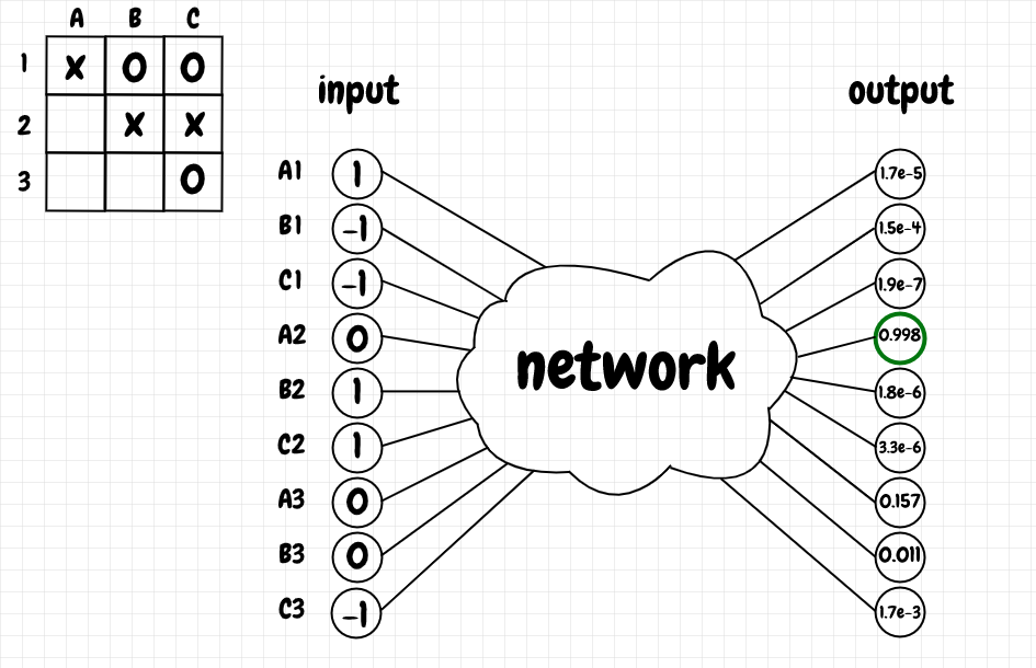
For the input into our network, we’ll flatten out the board position into an array of 9 values: 1 represents an X, -1 represents an O, and 0 is an empty cell. The output layer will be an array of 9 values representing the Q-value for each possible move: Something close to 0 represents a loss and a value close to 1 represents a win or a draw. After training, the network will choose the move corresponding to the highest output value from this model.
The diagram below shows the input and output for the given position after training (initially all of the values hover around 0.5):

As we can see, the winning move for X, A2, has the highest Q-value, 0.998, and the illegal moves have very low Q-values. The Q-values for the other legal moves are greater than the illegal ones, but less than the winning move. That’s what we want.
Model
The network (using PyTorch) has the following structure:
class TicTacNet(nn.Module):
    def __init__(self):
        super().__init__()
        self.dl1 = nn.Linear(9, 36)
        self.dl2 = nn.Linear(36, 36)
        self.output_layer = nn.Linear(36, 9)

    def forward(self, x):
        x = self.dl1(x)
        x = torch.relu(x)

        x = self.dl2(x)
        x = torch.relu(x)

        x = self.output_layer(x)
        x = torch.sigmoid(x)
        return x
The 9 input values that represent the current board position are passed through two dense hidden layers of 36 neurons each, then to the output layer, which consists of 9 values, each corresponding to the Q-value for a given move
Training
Most of the training logic for this agent is the same as for the Q-table implementation discussed earlier in this series. However, in that implementation, we prevented illegal moves. For the neural network, I decided to teach it not to make illegal moves, so as to have a more realistic set of output values for any given position.
The code below, from qneural.py, shows how the parameters of the network are updated for a single training game:
def update_training_gameover(net_context, move_history, q_learning_player,
                             final_board, discount_factor):
    game_result_reward = get_game_result_value(q_learning_player, final_board)

    # move history is in reverse-chronological order - last to first
    next_position, move_index = move_history[0]

    backpropagate(net_context, next_position, move_index, game_result_reward)

    for (position, move_index) in list(move_history)[1:]:
        next_q_values = get_q_values(next_position, net_context.target_net)
        qv = torch.max(next_q_values).item()

        backpropagate(net_context, position, move_index, discount_factor * qv)

        next_position = position

    net_context.target_net.load_state_dict(net_context.policy_net.state_dict())


def backpropagate(net_context, position, move_index, target_value):
    net_context.optimizer.zero_grad()
    output = net_context.policy_net(convert_to_tensor(position))

    target = output.clone().detach()
    target[move_index] = target_value
    illegal_move_indexes = position.get_illegal_move_indexes()
    for mi in illegal_move_indexes:
        target[mi] = LOSS_VALUE

    loss = net_context.loss_function(output, target)
    loss.backward()
    net_context.optimizer.step()
We maintain two networks, the policy network (policy_net) and the target network (target_net). We perform backpropagation on the policy network, but we obtain the maximum Q-value for the next state from the target network. That way, the Q-values obtained from the target network aren’t changing during the course of training for a single game. Once we complete training for a game, we update the target network with the parameters of the policy network (load_state_dict).
move_history contains the Q-learning agent’s moves for a single training game at a time. For the last move played by the Q-learning agent, we update its chosen move with the reward value for that game - 0 for a loss, and 1 for a win or a draw. Then we go through the remaining moves in the game history in reverse-chronological order. We tug the Q-value for the move that was played in the direction of the maximum Q-value from the next state (the next state is the state that results from the action taken in the current state).
This is analogous to the exponential moving average used in the tabular Q-learning approach: In both cases, we are pulling the current value in the direction of the maximum Q-value available from the next state. For any illegal move from a given game position, we also provide negative feedback for that move as part of the backpropagation. That way, our network will hopefully learn not to make illegal moves.
Results
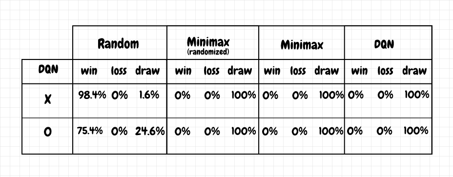
The results are comparable to the tabular Q-learning agent. The following table (based on 1,000 games in each case) is representative of the results obtained after a typical training run:

These results were obtained from a model that learned from 2 million training games for each of X and O (against an agent making random moves). It takes over an hour to train this model on my PC. That’s a huge increase over the number of games needed to train the tabular agent.
I think this shows how essential large amounts of high-quality data are for deep learning, especially when we go from a toy example like this one to real-world problems. Of course the advantage of the neural network is that it can generalize - that is, it can handle inputs it has not seen during training (at least to some extent).
With the tabular approach, there is no interpolation: The best we can do if we encounter a position we haven’t seen before is to apply a heuristic. In games like go and chess, the number of positions is so huge that we can’t even begin to store them all. We need an approach which can generalize, and that’s where neural networks can really shine compared to prior techniques.
Our network offers the same reward for a win as for a draw. I tried giving a smaller reward for a draw than a win, but even lowering the value for a draw to something like 0.95 seems to reduce the stability of the network. In particular, playing as X, the network can end up losing a significant number of games against the randomized minimax agent. Making the reward for a win and a draw the same seems to resolve this problem.
Even though we give the same reward for a win and a draw, the agent seems to do a good job of winning games. I believe this is because winning a game usually ends it early, before all 9 cells on the board have been filled. This means there is less dilution of the reward going back through each move of the game history (the same idea applies for losses and illegal moves). On the other hand, a draw requires (by definition) all 9 moves to be played, which means that the rewards for the moves in a given game leading to a draw are more diluted as we go from one move to the previous one played by the Q-learning agent. Therefore, if a given move consistently leads to a win sooner, it will still have an advantage over a move that eventually leads to a draw.
Network Topology and Hyperparameters
As mentioned earlier, this model has two hidden dense layers of 36 neurons each. MSELoss is used as the loss function and the learning rate is 0.1. relu is used as the activation function for the hidden layers. sigmoid is used as the activation for the output layer, to squeeze the results into a range between 0 and 1.
Given the simplicity of the network, this design may seem self-evident. However, even for this simple case study, tuning this network was rather time consuming. At first, I tried using tanh (hyperbolic tangent) for the output layer - it made sense to me to set -1 as the value for a loss and 1 as the value for a win. However, I was unable to get stable results with this activation function. Eventually, after trying several other ideas, I replaced it with sigmoid, which produced much better results. Similarly, replacing relu with something else in the hidden layers made the results worse.
I also tried several different network topologies, with combinations of one, two, or three hidden layers, and using combinations of 9, 18, 27, and 36 neurons per hidden layer. Lastly, I experimented with the number of training games, starting at 100,000 and gradually increasing that number to 2,000,000, which seems to produce the most stable results.
DQN
This implementation is inspired by DeepMind’s DQN architecture (see Human-level control through deep reinforcement learning), but it’s not exactly the same. DeepMind used a convolutional network that took direct screen images as input. Here, I felt that the goal was to teach the network the core logic of tic-tac-toe, so I decided that simplifying the representation made sense. Removing the need to process the input as an image also meant fewer layers were needed (no layers to identify the visual features of the board), which sped up training.
DeepMind’s implementation also used experience replay, which applies random fragments of experiences as input to the network during training. My feeling was that generating fresh random games was simpler in this case.
Can we call this tic-tac-toe implementation “deep” learning? I think this term is usually reserved for networks with at least three hidden layers, so probably not. I believe that increasing the number of layers tends to be more valuable with convolutional networks, where we can more clearly understand this as a process where each layer further abstracts the features identified in the previous layer, and where the number of parameters is reduced compared to dense layers. In any case, adding layers is something we should only do if it produces better results.
Code
The full code is available on github (qneural.py and main_qneural.py):
Experimenting with different techniques for playing tic-tac-toe
Demo project for different approaches for playing tic-tac-toe.
Code requires python 3, numpy, and pytest. For the neural network/dqn implementation (qneural.py), pytorch is required.
Create virtual environment using pipenv:
Install using pipenv:
pipenv shellpipenv install --dev
Set PYTHONPATH to main project directory:
- In windows, run
path.bat
- In bash run
source path.sh
Run tests and demo:
- Run tests:
pytest
- Run demo:
python -m tictac.main
- Run neural net demo:
python -m tictac.main_qneural
Latest results:
C:\Dev\python\tictac>python -m tictac.main
Playing random vs random:
-------------------------
x wins: 60.10%
o wins: 28.90%
draw  : 11.00%

Playing minimax not random vs minimax random:
---------------------------------------------
x wins: 0.00%
o wins: 0.00%
draw  : 100.00%

Playing minimax random vs minimax not random:
---------------------------------------------
x wins: 0.00%
o wins: 0.00%
draw  : 100.00%

Playing minimax not random vs minimax not random:
-------------------------------------------------
x wins: 0.00%
o wins: 0.00%
draw  : 100.00%

Playing minimax random vs minimax random:
-----------------------------------------
x wins: 0.00%
o wins: 0.00%
draw  : 100.00%

Playing minimax random vs random:
---------------------------------
x wins: 96.80%
o wins: 0.00%
draw  : 3.20%

Playing random vs minimax random:
---------------------------------
x wins: 0.00%
o wins: 78.10%
draw  : 21.90%

Training qtable X vs. random...
700/7000 games, using epsilon=0.6...
1400/7000 games, using epsilon=0.5...
2100/7000 games, using epsilon=0.4...
2800/7000 games, using epsilon=0.30000000000000004...
3500/7000 games, using epsilon=0.20000000000000004...
4200/7000 games, using epsilon=0.10000000000000003...
4900/7000 games, using epsilon=2.7755575615628914e-17...
5600/7000 games, using epsilon=0...
6300/7000 games, using epsilon=0...
7000/7000 games, using epsilon=0...
Training qtable O vs. random...
700/7000 games, using epsilon=0.6...
1400/7000 games, using epsilon=0.5...
2100/7000 games, using epsilon=0.4...
2800/7000 games, using epsilon=0.30000000000000004...
3500/7000 games, using epsilon=0.20000000000000004...
4200/7000 games, using epsilon=0.10000000000000003...
4900/7000 games, using epsilon=2.7755575615628914e-17...
5600/7000 games, using epsilon=0...
6300/7000 games, using epsilon=0...
7000/7000 games, using epsilon=0...

Playing qtable vs random:
-------------------------
x wins: 93.10%
o wins: 0.00%
draw  : 6.90%

Playing qtable vs minimax random:
---------------------------------
x wins: 0.00%
o wins: 0.00%
draw  : 100.00%

Playing qtable vs minimax:
--------------------------
x wins: 0.00%
o wins: 0.00%
draw  : 100.00%

Playing random vs qtable:
-------------------------
x wins: 0.00%
o wins: 61.00%
draw  : 39.00%

Playing minimax random vs qtable:
---------------------------------
x wins: 0.00%
o wins: 0.00%
draw  : 100.00%

Playing minimax vs qtable:
--------------------------
x wins: 0.00%
o wins: 0.00%
draw  : 100.00%

Playing qtable vs qtable:
-------------------------
x wins: 0.00%
o wins: 0.00%
draw  : 100.00%

number of items in qtable = 747

Training MCTS...
400/4000 playouts...
800/4000 playouts...
1200/4000 playouts...
1600/4000 playouts...
2000/4000 playouts...
2400/4000 playouts...
2800/4000 playouts...
3200/4000 playouts...
3600/4000 playouts...
4000/4000 playouts...

Playing random vs MCTS:
-----------------------
x wins: 0.00%
o wins: 63.50%
draw  : 36.50%

Playing minimax vs MCTS:
------------------------
x wins: 0.00%
o wins: 0.00%
draw  : 100.00%

Playing minimax random vs MCTS:
-------------------------------
x wins: 0.00%
o wins: 0.00%
draw  : 100.00%

Playing MCTS vs random:
-----------------------
x wins: 81.80%
o wins: 0.00%
draw  : 18.20%

Playing MCTS vs minimax:
------------------------
x wins: 0.00%
o wins: 0.00%
draw  : 100.00%

Playing MCTS vs minimax random:
-------------------------------
x wins: 0.00%
o wins: 0.00%
draw  : 100.00%

Playing MCTS vs MCTS:
---------------------
x wins: 0.00%
o wins: 0.00%
draw  : 100.00%
C:\Dev\python\tictac>python -m tictac.main_qneural
Training qlearning X vs. random...
200000/2000000 games, using epsilon=0.6...
400000/2000000 games, using epsilon=0.5...
600000/2000000 games, using epsilon=0.4...
800000/2000000 games, using epsilon=0.30000000000000004...
1000000/2000000 games, using epsilon=0.20000000000000004...
1200000/2000000 games, using epsilon=0.10000000000000003...
1400000/2000000 games, using epsilon=2.7755575615628914e-17...
1600000/2000000 games, using epsilon=0...
1800000/2000000 games, using epsilon=0...
2000000/2000000 games, using epsilon=0...
Training qlearning O vs. random...
200000/2000000 games, using epsilon=0.6...
400000/2000000 games, using epsilon=0.5...
600000/2000000 games, using epsilon=0.4...
800000/2000000 games, using epsilon=0.30000000000000004...
1000000/2000000 games, using epsilon=0.20000000000000004...
1200000/2000000 games, using epsilon=0.10000000000000003...
1400000/2000000 games, using epsilon=2.7755575615628914e-17...
1600000/2000000 games, using epsilon=0...
1800000/2000000 games, using epsilon=0...
2000000/2000000 games, using epsilon=0...

Playing qneural vs random:
--------------------------
x wins: 98.40%
o wins: 0.00%
draw  : 1.60%

Playing qneural vs minimax random:
----------------------------------
x wins: 0.00%
o wins: 0.00%
draw  : 100.00%

Playing qneural vs minimax:
---------------------------
x wins: 0.00%
o wins: 0.00%
draw  : 100.00%

Playing random vs qneural:
--------------------------
x wins: 0.00%
o wins: 75.40%
draw  : 24.60%

Playing minimax random vs qneural:
----------------------------------
x wins: 0.00%
o wins: 0.00%
draw  : 100.00%

Playing minimax vs qneural:
---------------------------
x wins: 0.00%
o wins: 0.00%
draw  : 100.00%

Playing qneural vs qneural:
---------------------------
x wins: 0.00%
o wins: 0.00%
draw  : 100.00%
References


